I recently tweeted a chart that showed the P/E ratio of various countries’ equity markets relative to the volatility of earnings growth in that country. There was a correlation: lower earnings volatility tended to result in a higher P/E ratio. This prompted an interesting question—what does a P/E ratio tell you about investor expectations?

There is a strong correlation between low earnings growth volatility and higher P/E ratios, with some outliers (China looks a bit suspicious). Note that emerging mkts have US-like volatility in earnings, but with considerably lower valuations (Canada, as well).
(src @fathommacro) pic.twitter.com/J2ZySLAYY5

— Franklin J. Parker, CFA (@FranklinParker1) February 9, 2022

I am a big fan of extracting market expectations on various questions. It can give a starting point for your own analysis, giving a sort of “benchmark of knowledge” on a question. Here is what the market thinks, do I agree with that? If I do not agree, why not? Do I have more evidence/insight than the market or should I just adopt that view?

So, what can a P/E ratio tell us about investor expectations? Just for fun, let’s get creative with the math of the topic to see what we can see!

The price-to-earnings ratio is pretty self explanatory—we take the current price of a company and divide by the current earnings of a company (or market). Earnings are also self-explanatory.

Price, however, can be broken down a bit further. If we think of a stock as a growing series of cashflows, we can use the formula for a growing perpetuity to define our price:

where r is our discount rate and g is the growth rate of the cashflows. E is current earnings, so the numerator gives us next year’s earnings expectation.

A quick point on the discount rate. This is not the risk-free rate. This is a volatility-adjusted discount rate, and it must be greater than the growth rate of the cashflows. As a shorthand, you could think of it as discount rate = growth rate + volatility of growth rate. Then, r will always be greater than g.

If we put this in for price in our P/E ratio:

Simplifying to

If, then, you know the market’s required return and the stock’s P/E, you can extract the market’s earnings growth expectation:

Or, if you know the market’s growth expectation and the stock’s P/E, you can extract the market’s discount rate:

So, what does the P/E ratio tell you about a stock or market?

• P/E ratios tell you the market’s expected earnings growth, if you know the market’s discount rate.
• P/E ratios tell you the market’s discount rate, if you know the market’s expected growth rate.

Clearly there is a bit of recursion here, because we don’t know either variable in practice. However, relationship can give us a sense of acceptable combinations of the two.

Using R, let’s illustrate how these interplay. We’ll need the tidyverse and rgl libraries.

Let’s take the above relationships and convert them to R functions

# Resultant growth rate, given a required return & P/E ratio
g.f <- function(r, P_E){
  (P_E * r - 1)/(1 + P_E)
}
# Resultant required return, given an expected growth rate & P/E ratio
r.f <- function(g, P_E){
  (1 + g)/P_E + g
}
# Resultant P/E ratio, given growth rate and required return
PE.f <- function(g, r){
  (1 + g)/(r - g)
}

Let’s visulize how P/E is affected by the two main inputs, discount rate and expected growth rate.

# Simulate values of r and g
r <- seq(-0.10, 0.10, 0.001)
g <- seq(-0.10, 0.10, 0.001)
# Find resultant P/E ratio
PE.mat <- matrix( nrow = length(r), 
                  ncol = length(g) )
for(i in 1:length(r)){
  for(j in 1:length(g)){
    PE.mat[i,j] <- PE.f( g[j], r[i])
  }
}
# Remove r < g scenarios
PE.mat[ which(PE.mat <= 0) ] <- NA
# Replace infinite values with N/A
PE.mat[ !is.finite( PE.mat ) ] <- NA
rownames(PE.mat) <- r
colnames(PE.mat) <- g
# Visulize how g and r yield various P/Es
persp3d( x = r,
        y = g,
        z = PE.mat,
        col = 'dodgerblue',
        zlim = c(0,100),
        xlab = 'Discount Rate',
        ylab = 'Growth Rate',
        zlab = 'P/E Ratio')

Giving us a cool plot that we can grab and turn at will (thank you rgl library!).

Of course, the graph is asymptotic with respect to r = g, because at that point the divisor is 0.

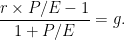
Taking some more helpful cross-sections of the plot above, we can see how growth rates and required returns interact, given an observable P/E ratio. While we do not know which combination is the market’s solution, we can at least get some ballparks.

data.frame( 'E.Growth' = c(g.f(r, 28),
                           g.f(r, 18),
                           g.f(r, 38) ),
            'Req.Return' = c(r, r, r),
            'PE' = c( rep('28', length(r)),
                      rep('18', length(r)),
                      rep('38', length(r)) ) ) %>% 
  ggplot(., aes(x = Req.Return, y = E.Growth, col = PE))+
  geom_line( size = 1.25 )+
  xlab('Discount Rate')+
  ylab('Expected Growth')+
  theme_minimal()

Yielding

Which shows us that the tradeoff between growth and the discount rate is linear!

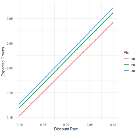
But there are other, more useful, ways to slice these relationships. Let’s look at how changes in expected growth rates shift P/E ratios (and vice versa).

In this first plot we hold the discount rate constant at r = 0.12 and show how P/E is an exponential function of expected growth rates.

data.frame( 'E.Growth' = g,
            'PE' = PE <- PE.f(g, 0.12) ) %>% 
  ggplot(., aes(x = E.Growth, y = PE))+
  geom_line( size = 1.25 )+
  xlab('Expected Growth Rate')+
  ylab('P/E Ratio')+
  theme_minimal()

This is a helpful way to view changes in P/E ratios and/or growth rates. If, for example, you witness the P/E ratio of a stock (or market) move from 25 to 15 (keeping the assumed discount rate the same), then you can infer that the market has adjusted its expected growth rate on the business from 7.5% to 5%.

You can also use this as a way to intelligently disagree with markets. If, for example, you believe a business (or market) will shift their growth rate from 10% to 5%, but the market has only moved the P/E ratio from 60 to 50, you might argue that the business is still overvalued, even though it has already lost price.

As we mentioned earlier, the graph is asymptotic with respect to r = g, and exponential up to that point, which means that estimating the risk-adjusted discount rate is pretty critical to any analysis—a point I have largely hand-waved away. Unfortunately, this is not an observable value, and estimation of several variables will be critical!

If you take the very simplistic view of the volatility-adjusted discount that I just mentioned (r = g + s(g)), the whole analysis becomes linear, which is both exciting and suspicious!

Or, the P/E ratio is simply the earnings growth rate discounted by the volatility of those earnings.

I would throw a flag on this simplification were I you, but it does both simplify the idea and passes the sniff test—at least to me. Consider this:

data.frame( 's' = s <- seq(0.015, 0.25, 0.001),
            'PE' = (1.08/s) ) %>% 
  ggplot(., aes(x = s, y = PE))+
  geom_line( size = 1.25 )+
  xlab('Volatility of Earnings Growth')+
  ylab('P/E Ratio')+
  theme_minimal()

See how valuations increase as volatility decreases? That makes sense, and is supported by the plot at the very top of the post. (Of course, in practice, growth rates also decrease as volatility decreases—I kept growth rates constant in the plot).

Now, I have to caution all of us against such simplistic models of the world. While these relationships are a little bit true, it is also true that investors are constantly forced to make tradeoffs across potential investments. That means that TINA (there is nothing else) is a real thing, as is the infusion of easy money, etc.

The point is, the world is complex and a very simple model like this should only serve to further our intuition on a topic, not define the topic entirely. Even so, it does appear there is some information to be gained from observed P/E ratios.

But, as always, do your own research (and share it with me when you do)!