
RObservations #25: Using R and Stan to Estimate Ad Effectiveness
Want to share your content on R-bloggers? click here if you have a blog, or here if you don't.

Introduction
Recently, I have started taking a course on Bayesian statistics and using Stan– a fast language designed specifically for preforming the simulations necessary for Bayesian analysis by employing Markov-Chain Monte Carlo (MCMC) algorithms. While it may sound abstract, thousands of users rely on Stan for statistical modeling, data analysis, and prediction in the social, biological, and physical sciences, engineering, and business (as claimed by the website). On the Stan Youtube channel there is a video of a “toy example” showing how it is possible to do split testing on social media outlets to determine ad-effectiveness as measured through click-through rate (CTR).
In the toy example, 10 impressions are bought to advertise on Facebook and Twitter. While it may first look that Twitter is a better outlet, implementing Stan to create the posterior distributions of the advertising CTR on each social media outlet shows that the actual uncertainty (represented by the spread of the distributions) is still quite large and could be accredited to chance. In the end it is shown that Facebook is a truly better platform and it could be hinted to from the posterior distributions.
While this all looks great, it got me thinking, does this hold up with real data? After making a post on LinkedIn and reaching out to some of my connections in digital marketing, my colleague Max Kalles, owner at Smarter Leads sent me some data from an ad campaign he ran 2 years ago on a variety of platforms (Google, Bing, Facebook and Pintrest).
In this blog I will attempt to estimate the the distribution of the CTR on the platforms Max ran his ad campaign using Stan and the rstan package and see if the results created are insightful and informative for what what the true CTR was for that year actually turned out to be on the platforms he ran the campaigns.
Setting up the simulation
The data I got from Max is different from the example from the Stan Youtube Channel because it is much larger in sample size and I don’t know the result of each individual impression. However, since the real world is often not like how it is shown in the examples, lets deal with it analyze accordingly.
The data for the first month of the campaign is:
firstMonthData <- data.frame(channel=c("Google",
                                       "Bing",
                                       "Facebook",
                                       "Pintrest"),
                             impressions=c(37821,
                                           11635,
                                           245690,
                                           407012),
                             clicks = c(1787,
                                        460,
                                        1847,
                                        1717))

within(firstMonthData,{ctr<- clicks/impressions})


##    channel impressions clicks         ctr
## 1   Google       37821   1787 0.047248883
## 2     Bing       11635    460 0.039535883
## 3 Facebook      245690   1847 0.007517603
## 4 Pintrest      407012   1717 0.004218549
Now that we have the data for the first month we can proceed with working with Stan. As was the case with the toy example I will be having my priors being set as uniform. The Stan code implemented is:
data{
  // Number of impressions
  int n1;
  int n2;
  int n3;
  int n4;

  // number of clicks

  int y1[n1];
  int y2[n2];
  int y3[n3];
  int y4[n4];

}

parameters{
  // Prior Parameters
  real<lower=0, upper=1> theta1;
  real<lower=0, upper=1> theta2;
  real<lower=0, upper=1> theta3;
  real<lower=0, upper=1> theta4;
}

// Prior distribution
model{
  // All have uniform priors
  theta1 ~ beta(1,1);
  theta2 ~ beta(1,1);
  theta3 ~ beta(1,1);
  theta4 ~ beta(1,1);


  // Likelihood Functions
  y1~ bernoulli(theta1);
  y2 ~ bernoulli(theta2);
  y3~ bernoulli(theta3);
  y4~ bernoulli(theta4);
}
Since we do not know which impressions were clicked, assuming that the impressions which are clicked is random, lets create fake data representing each individual impression and randomly selecting which impression is clicked. The code to do this is listed below:
# Setting seed for reproducibility
set.seed(1234)

# Make a vector of 0's representing the impressions
y_google<-rep(0,37821)
# Randomly select impressions and assign them as clicked- the same number as the known data.
y_google[sample(c(1:37821),1787)] <- 1
# Now lets do it for the rest of the data
y_bing<-rep(0,11635)
y_bing[sample(c(1:11635),460)]<-1

y_facebook<-rep(0,245690)
y_facebook[sample(c(1:245690),1847)]<-1

y_pintrest<-rep(0,407012)
y_pintrest[sample(c(1:407012),1717)]<-1
Now that the data has been created, lets put Stan to work!
library(rstan)

# Set up the data in list form
data <- list(n1=length(y_google),
             n2=length(y_bing),
             n3= length(y_facebook),
             n4=length(y_pintrest),
             y1=y_google,
             y2=y_bing,
             y3=y_facebook,
             y4=y_pintrest)

fit <- stan(file ="./stanMarketingCode.stan",
            data=data)
Now that Stan has done the work for us we can see how are results faired in the visuals below:
library(tidyverse)
library(reshape2)
library(ggthemes)
library(ggpubr)

rstan::stan_plot(fit)+
  ggtitle("Density of Posterior Distribution of CTR by Channel")

params<- rstan::extract(fit) %>%
         as.list() %>%
         as_tibble() %>%
         select(!lp__) %>%
         transmute("Google CTR (theta1)"= theta1,
                   "Bing CTR (theta2)" = theta2,
                   "Facebook CTR (theta3)"= theta3,
                   "Pintrest CTR (theta4)"=theta4) %>%
        melt() %>%
        mutate(value=c(value))

ggplot(data=params,
       mapping=aes(x=value,fill=variable))+
  geom_density(alpha=0.5)+
  theme_light()+
  theme(legend.title = element_blank(),
        legend.position = "bottom")+
  ggtitle("Density of Posterior Distribution of CTR by Channel")
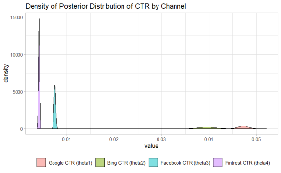
While it can be seen that the distributions of the CTR across channels are centered around their analytical CTR. The distributions visualized enable us to see the uncertainty in those results. Max ran a this campaign with some large numbers so the hierarchy of Google > Bing > Facebook > Pinterest in terms of CTR is largely apparent.
Comparing this result to the real world data.
From the real world data that I got from Max, the CTR for all the channels are:
allData<- data.frame(channel=c("Google",
                                       "Bing",
                                       "Facebook",
                                       "Pintrest"),
                             impressions=c(1221362,
                                           59105,
                                           5227042,
                                           407012),
                             clicks = c(59105,
                                        2251,
                                        31566,
                                        1717))

within(allData, {ctr<-clicks/impressions})


##    channel impressions clicks         ctr
## 1   Google     1221362  59105 0.048392696
## 2     Bing       59105   2251 0.038084764
## 3 Facebook     5227042  31566 0.006038980
## 4 Pintrest      407012   1717 0.004218549
Which fall within the distributions that we estimated with Stan.
Conclusion
This simulation might have been superfluous as the size of the overall campaigns where much larger and likely gave the effectiveness of the ad campaigns from the initial CTR generated. Had the data been smaller the lines could have possibly been blurred as to what the the superior channel for this campaign was.
Nevertheless, this was a good exercise in how a Bayesian analysis would look like as far as viewing raw data points in terms of a distribution as opposed to just their face value, and for that I am happy to have seen that.
![]()
Once again, be sure to check out Smarter Leads for all your digital marketing needs. Thank you Max for sending me this data!

Want to see more of my content?
Be sure to subscribe and never miss an update!
R-bloggers.com offers daily e-mail updates about R news and tutorials about learning R and many other topics. Click here if you're looking to post or find an R/data-science job.
Want to share your content on R-bloggers? click here if you have a blog, or here if you don't.