Until today, we have examined the supervised learning algorithms; but this time, we will take a look at a different learning method. The algorithm we just mentioned is association rules which is an unsupervised learning method. The algorithm is referred to as market basket analysis as it usually has been applied to grocery data.

The market basket analysis has the items, which are in the brackets, to form the itemset for each transaction(e.g. ). The association rules create the formation of itemsets as shown below:

This association rule indicates that if butter and jam are purchased together, then the bread is most likely to be purchased too. Since the association rule is unsupervised the data does not need to be labeled. These rules are created from subsets of itemsets that on the left-hand side (LHS) denotes the condition that needs to be met, and the right-hand side (RHS) indicates the expected outcome of meeting that condition.

In order to mine association rules algorithms among massive transactional data, we will use the apriori algorithm. This algorithm works on the concept that frequent itemsets can only be frequent if both components(items) of itemsets are frequent separately. Hence an itemset that has rare items would be extracted from the search.

The apriori algorithm uses some thresholds measurements which are called support and confidence measures to reduce the number of rules. The support of itemset or rule measures the frequency of it in the data.

• N is the number of transactions.
• is the number of transactions which contain that itemset.

The confidence measures the power of a rule; the closer to 1, the stronger the relationship of a rule. The support of the itemset which contains both X and Y is divided by the support of itemset containing only X, as shown below:

The Apriori algorithm uses the minimum support threshold to determine all potential itemsets and builds rules with the minimum confidence level. Besides all of that, we will use a different measurement to evaluate the rank of importance of the association rules, which indicates true connections between items.

The metric we’ve just mentioned is the Lift, which measures how much more likely it is that the items in the itemset are found together to the rate being alone.

To examine all concepts, we mentioned so far, we will examine the grocery data from the arules package. Let’s take a look first three transactions of the market basket data. The data is stored in sparse matrix format, as seen below. This matrix format stores only the items which are present and removes the missing cells to save the memory.

library(arules)
library(tidyverse)
library(scales)
library(glue)
library(ggiraph)
library(ggiraphExtra)

data("Groceries")

Groceries

#transactions in sparse format with
# 9835 transactions (rows) and
# 169 items (columns)

Groceries %>% 
  .[1:3] %>% 
  inspect()

#    items                 
#[1] {citrus fruit,        
#     semi-finished bread, 
#     margarine,           
#     ready soups}         
#[2] {tropical fruit,      
#     yogurt,              
#     coffee}              
#[3] {whole milk} 

Before mining the rules, we will look at the supports(frequencies) rates of the items for each. We will get the ones greater than 0.1 for a readable chart.

#frequency/support plot
Groceries %>% 
  itemFrequency() %>% 
  as_tibble(rownames = "items") %>% 
  rename("support"="value") %>% 
  filter(support >= 0.1) %>% 
  arrange(-support) %>% 
  ggDonut(aes(donuts=items,count=support),
          explode = c(2,4,6,8),
          labelposition=0)

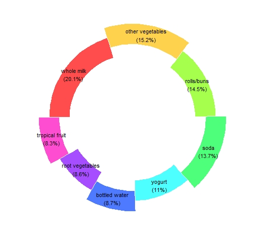
The whole milk appears to be the most frequent item in all transactions. Let’s see if this superiority is reflected in the association rules.

#Mining rules
groceryrules <- 
  Groceries %>% 
  apriori(parameter = list(
    support =0.006, 
    minlen = 2, 
    confidence=0.25))
  

#Rules plot
gg_rules <- 
  groceryrules %>% 
  arules::sort(by="lift") %>% 
  DATAFRAME() %>% 
  as_tibble() %>% 
  head(10) %>%
  mutate(ruleName = paste(LHS,"=>",RHS) %>% fct_reorder(lift),
         support = support %>% percent(),
         lift = lift %>% round(2)) %>%
  select(ruleName, support, lift) %>%  
  ggplot(aes(x=ruleName,y=lift))+
  geom_segment(aes(xend=ruleName, yend=0), 
               color="orange",
               size=1) +
  geom_point_interactive(aes(tooltip=glue("Support: {support}\nLift: {lift}"), 
                             data_id=support),
                         size=3, 
                         color="lightblue") +
  coord_flip() +
  theme_minimal() +
  theme(
    panel.grid.minor.y = element_blank(),
    panel.grid.major.y = element_blank(),
    panel.grid.minor.x = element_blank(),
    panel.background = element_rect(fill = "#e0ddd7", color = NA),
    plot.background = element_rect(fill = "#f5cecb", color = NA)
  ) +
  xlab("") +
  ylab("")

girafe(ggobj = gg_rules)

In the above code chunk, we have employed the apriori function to find the association rules, and we have sorted the rules by top 10 lift values. When we hoover on the blue points the pop-pup(tooltip) displays the lift and support values. This interactivity of the plot was provided by the ggiraph package.

The up top rule indicates the probability that those who buy herbs would also buy root vegetables is about four times more likely than buying root vegetables alone. The support value in the tooltip indicates the frequency of the rule, not the frequency of the itemsets.

References

• Lantz, Brett (2015). Machine Learning with R: Packt Publishing
• LOLLIPOP CHART