
Pastor and Stambaugh (2003) Liquidity Measure – Individual Stock
[This article was first published on K & L Fintech Modeling, and kindly contributed to R-bloggers]. (You can report issue about the content on this page here)
Want to share your content on R-bloggers? click here if you have a blog, or here if you don't.
This post shows how to calculate the liquidity measure (gamma) of Pastor and Stambaugh (2003) using R code. For exposition purposes we use only two individual series : small firm index and ESG firm index. As expected, a PS liquidity measure for small firms is more volatile than that of ESG firms. Want to share your content on R-bloggers? click here if you have a blog, or here if you don't.
Pastor and Stambaugh (2003) Liquidity Measure
According to Pastor and Stambaugh (2003), the individual stock’s monthly liquidity measure is constructed by estimating \(\color{blue}{\gamma_{?,?}} \) using the following regression model.
\[\begin{align} ?_{?,?+1,?}^? = \theta_{?,?}+\phi_{?,?} ?_{?,?,?}+ \color{blue}{\gamma_{?,?}} \color{red}{\text{????}(?_{?,?,?}^? )}\color{green}{v_{?,?,?}}+\epsilon_{?,?+1,?} \end{align}\]
\(?_{?,?,?}\) : the return on stock i on day d in month t, total return
\(?_{?,?,?}\) : the return on the market return on day d in month t
\(?_{?,?,?}^? : ?_{?,?,?}− ?_{?,?,?}\) : the return in excess of the market,
\(v_{?,?,?}\) : the dollar volume for stock i on day d in month t
\(sign()\) : sign indicator function (+,-)
By aggregating above estimates for all stocks, we construct the market-wide measure for each month. \[\begin{align} \hat{\gamma}_{?} = \frac{1}{N} \sum_{i=1}^N \hat{\gamma}_{?,?} \end{align}\] Since we cannot have access to a database which provides information of all stocks, instead we attempt to calculate two individual liquidity measures for expositional purpose and comparisons by using the above regression model.
Interpretation
Before going to R code, we need to understand the meaning of the above regression for individual stock’s liquidity measure. The basic idea is based on the strong volume-related return reversals.
Volume signed by the contemporaneous excess return on the stock should be accompanied by a return that one expects to be partially reversed in the future if the stock is not perfectly liquid. There is a tendency that when market liquidity drops today, risk-averse investors overreact to this negative shock today, which results in the large decrease in return today and the return reversal tomorrow.
In particular, the larger the trading volume, the smaller the magnitude of the return reversal in adverse times. It’s because higher trading volume mitigates decrease in stock prices. In other words, the greater the expected reversal for a given dollar volume, the lower the stock’s liquidity.
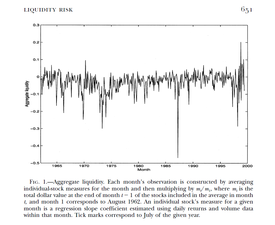
For reference, the published PS market-wide aggregate liquidity measure is as follows.
Data
If we have access to database which provide information of all stocks, we can calculate a market-wide liquidity measure using two equations. But we don’t have that access now, we calculate two liquidity measures of ESG index and small stock index for exercises.
It is known that better ESG-rated companies tend to have lower bid-ask spreads and more trading volume by enhancing the transparency and reducing the asymmetric information.For this reason, it deserves the comparisoin of these two stock index through the lens of the PS liquidity measure.
We assume KOSPI200 index as the market stock index which is used when we calculate the excess returns. Test data are two stock index : KOSPI200 ESG firms stock index and KOSPI200 small firms index.


R code
R code for PS liquidity measure performs monthly regressions repeatedly for each every month and generate a time series of \(\gamma_{it}\). R code is so simple since it only estimates a multiple regression with two explanatory variables with a constant term. For this estimation, we apply two methods : 1) split-apply-do.call and 2) lmList() function in lme4 R package. lmList() function performs a group-by regression.
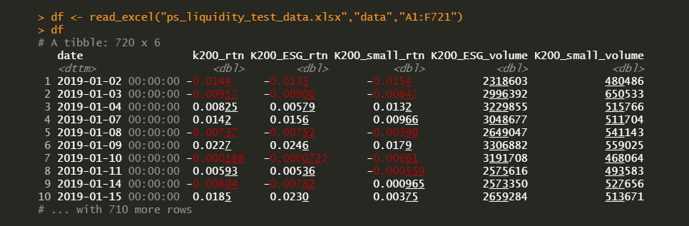
#========================================================# # Quantitative ALM, Financial Econometrics & Derivatives # ML/DL using R, Python, Tensorflow by Sang-Heon Lee # # https://kiandlee.blogspot.com #——————————————————–# # Pastor and Stambaugh (2003) liquidity measure #========================================================# graphics.off() # clear all graphs rm(list = ls()) # remove all files from your workspace library(readxl) library(lme4) setwd(“D:/SHLEE/blog/cross_section/ps_liquidity”) #—————————————————– # data specification #—————————————————– # date K200_rtn, K200_ESG_rtn, K200_small_rtn # K200_ESG_volume, K200_small_volume #—————————————————– df <– read_excel(“ps_liquidity_test_data.xlsx”,“data”,“A1:F721”) df # monthly group indicator df$yyyymm <– strftime(df$date,“%Y%m”) # returns in excess of market index df$ESG_ex_rtn <– df$ESG_rtn – df$K200_rtn df$small_ex_rtn <– df$small_rtn – df$K200_rtn # data for regression df.reg.data <– cbind(df[–nrow(df),], ESG_ex_rtn_y = df$ESG_ex_rtn[–1], small_ex_rtn_y = df$small_ex_rtn[–1]) #—————————————————– # regression for individual stock’s PS liquidity measure #—————————————————– #—————- # Method 1 #—————- # ESG firm index lt.esg.out <– lapply( split(df.reg.data, df.reg.data$yyyymm), # split function(x){ eq <– lm(ESG_ex_rtn_y ~ ESG_rtn + I(sign(ESG_ex_rtn)*ESG_volume), data=x) return(eq$coefficients) }) do.call(rbind,lt.esg.out) # concatenate rows # Small firm index lt.small.out <– lapply( split(df.reg.data, df.reg.data$yyyymm), # split function(x){ eq <– lm(small_ex_rtn_y ~ small_rtn + I(sign(small_ex_rtn)*small_volume), data=x) return(eq$coefficients) }) do.call(rbind,lt.small.out) # concatenate rows #—————- # Method 2 #—————- # ESG firm index esg.fits <– lmList( ESG_ex_rtn_y ~ ESG_rtn + I(sign(ESG_ex_rtn)*ESG_volume) | yyyymm, data=df.reg.data) coef(esg.fits) # Small firm index small.fits <– lmList( small_ex_rtn_y ~ small_rtn + I(sign(small_ex_rtn)*small_volume) | yyyymm, data=df.reg.data) coef(small.fits) | cs |
Results
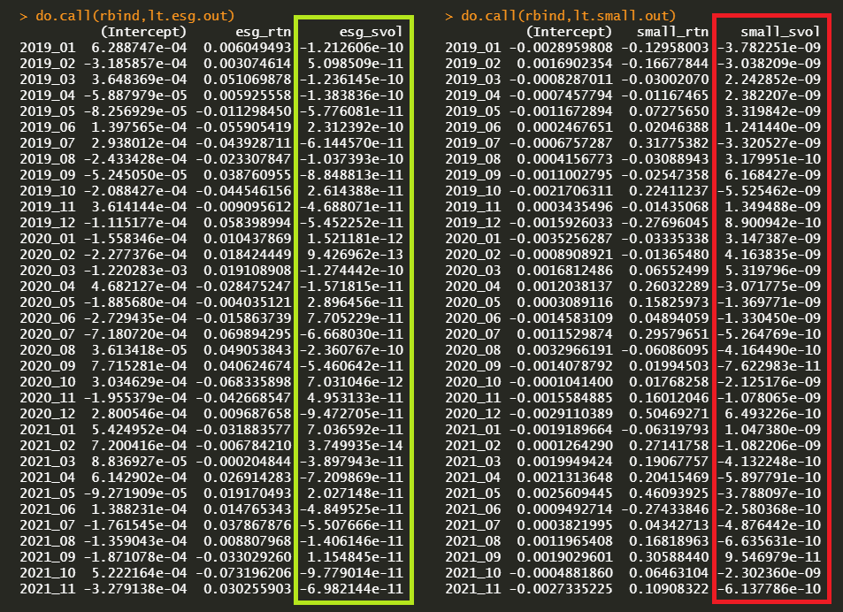
Regression parameter estimates are as follows (green color for ESG firm index and red color for small firm index).
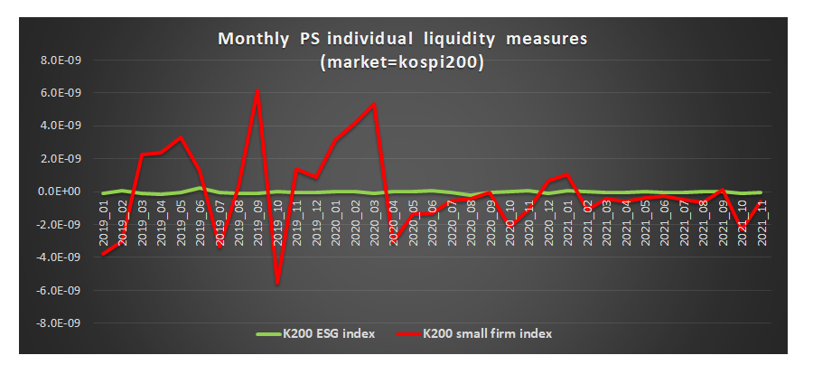
The following graph shows that the PS liquidity measure of small firm index is more volatile than that of ESG firm index as expected. But the PS liquidity measure of ESG index is too stable unexpectedly.
Concluding Remarks
In this post, we estimate the PS individual stock’s liquidity measure of two stock indices (ESG and small firm) for understanding the logic of Pastor and Stambaugh (2003). Although we do not have access to database which provides information of all stocks, we could have grasped the overall process using these simple example.
Small firm index showed volatile movements of the PS liquidity measure. But why did ESG index show too stable liquidity measure? it remains for further research.
Pástor, Ľ and R. F. Stambaugh (2003) Liquidity Risk and Expected Stock Returns, Journal of Political Economy 111-3, pp. 642-685. \(\blacksquare\)
Reference
Pástor, Ľ and R. F. Stambaugh (2003) Liquidity Risk and Expected Stock Returns, Journal of Political Economy 111-3, pp. 642-685. \(\blacksquare\)
To leave a comment for the author, please follow the link and comment on their blog: K & L Fintech Modeling.
R-bloggers.com offers daily e-mail updates about R news and tutorials about learning R and many other topics. Click here if you're looking to post or find an R/data-science job.
Want to share your content on R-bloggers? click here if you have a blog, or here if you don't.