This post explains how to use the augmented Dickey-Fuller (ADF) test in R. The ADF Test is a common statistical test to determine whether a given time series is stationary or not. We explain the interpretation of ADF test results from R package by making the meaning of the alphanumeric name of test statistics clear.

ADF test

We have implemented a R code for the VAR model in the prior post below but have not discussed the ADF test specifically, which is the test for stationarity or nonstationary (unit root) of a given time series. ADF test should be done before building up VAR or VECM model.

stationary and non-stationary

Roughly speaking, a stationary time series is one whose mean, variance and autocorrelation are all constant over time. In contrast, a time series is non-stationary when the these three statistics change over time. For example, a time series of GDP level is non-stationary but GDP growth (=log difference of GDP) is stationary. While the former exhibits a upward trend with increasing mean and variance, the latter does not.

ADF test

A distinction between stationary and non-stationary time series is made by formal statistical procedures such as ADF (Augmented Dickey-Fuller) test, which is frequently used since it account for serial correlation in time series (Dickey and Fuller; 1979). Three specifications of ADF test have the following regressions.
\[\begin{align} \Delta y_t &= \color{red}\gamma y_{t-1} + \underbrace{\sum_{i=2}^{p} \beta_i \Delta y_{t-i+1}}_\text{control for serial correlation} + \epsilon_t \\ \rightarrow (\tau1&)\quad H_0 : \color{red} {\gamma = 0} \\\\ \Delta y_t &= \color{red}{\gamma} y_{t-1} + \underbrace{\color{blue}{a_0}}_\text{constant} + \sum_{i=2}^{p} \beta_i \Delta y_{t-i+1} + \epsilon_t \\ \rightarrow (\phi1&)\quad H_0 : \color{red} {\gamma = 0} \quad\&\quad\color{blue}{a_0 = 0} \\\ \rightarrow (\tau2&)\quad H_0 : \color{red} {\gamma = 0} \\\ \Delta y_t &= \color{red}{\gamma} y_{t-1} + \color{blue}{a_0} + \underbrace{\color{green}{a_2} t}_{trend} + \sum_{i=2}^{p} \beta_i \Delta y_{t-i+1} + \epsilon_t \\ \rightarrow (\phi2&)\quad H_0 : \color{red} {\gamma = 0} \quad\&\quad \color{blue}{a_0 = 0} \quad\&\quad \color{green}{a_2 = 0} \\ \rightarrow (\phi3&)\quad H_0 : \color{red} {\gamma = 0} \quad\&\quad\color{blue}{a_0 = 0} \\ \rightarrow (\tau3&)\quad H_0 : \color{red} {\gamma = 0} \end{align}\]
Each test regression has one or more test statistics for the restrictions on some parameters which are of interest : \(\tau1\) in the 1st equation, \(\phi1\) and \(\tau2\) in the 2nd equation, \(\phi2\) and \(\phi3\) and \(\tau3\) in the 3rd equation. It is interesting that alphanumeric words for the name of test statistics are ordered from joint hypothesis to single hypothesis within each equation.

The above three equations are considered different so that test statistics are dependent on the specification of equations. This results in the unique numbers attached to \(\tau\) and \(\phi\) such as \(\tau1, \tau2, \tau3\) and \(\phi1,\phi2,\phi3\).

Put simply, \(\tau = 0\) indicates the presence of unit root. \(\phi1 = 0\) or \(\phi3 = 0\) denotes the presence of unit root and the absence of intercept. \(\phi2 = 0\) denotes the presence of unit root and the absence of intercept and trend.

The reason why test statistics are placed below its regressions with some ordering is that ADF result from R package follow this ordering and the name of test statistics. Without knowing these notations, it is a bit confusing to interpret R’s ADF output. So I simplified it for the easy understanding.

Which specifications do we select?

Constant term is usually included. When a time series show a trend, we just include a trend term. However, when we are not certain about the specification, we use all regression above and check the statistical significances of the test statistics.

As ADF test also deal with the serial correlation by introducing lagged terms of \(\Delta y_{t}\), we need to select this lag order. This is accomplished by investigating ACF, PACF or several informaiton criteria but we rely on an automatic lag selection functionality of R package.

Data

From urca R package, we can load denmark dataset which was used in the prior post. This dataset consists of logarithm of real money M2 (LRM), logarithm of real income (LRY), logarithm of price deflator (LPY), bond rate (IBO), bank deposit rate (IDE), which covers the period 1974:Q1 – 1987:Q3.

The plot of the data with an overlay of its own differenced data are shown in the next figure. When looking at the plot of each data, level variables show a trend except interest rates and its first difference does not show any trend.

ur.df : ADF test function in urca R library

ur.df() function urca R library performs the ADF unit root test, which has the next specification. In particular, when we use selectlags parameters, lag order of lagged dependent variable is automatically selected.

R code

In the following R code, we perform ADF test for denmark time series by using ur.df() function.



The ADF result for LRM variable from the above R code is generated as follows and our focus is on the yellow rectangular area which shows the ADF test result.

Interpretation

Interpretation of ADF test follow the general-to-specific approach. As such, three regression models are applied sequentially. For interpretation, let’s take LRY variable for example by using the following R code.



We can get the following summarized ADF test results for level and 1st difference variable of LRY (logarithm of real income).



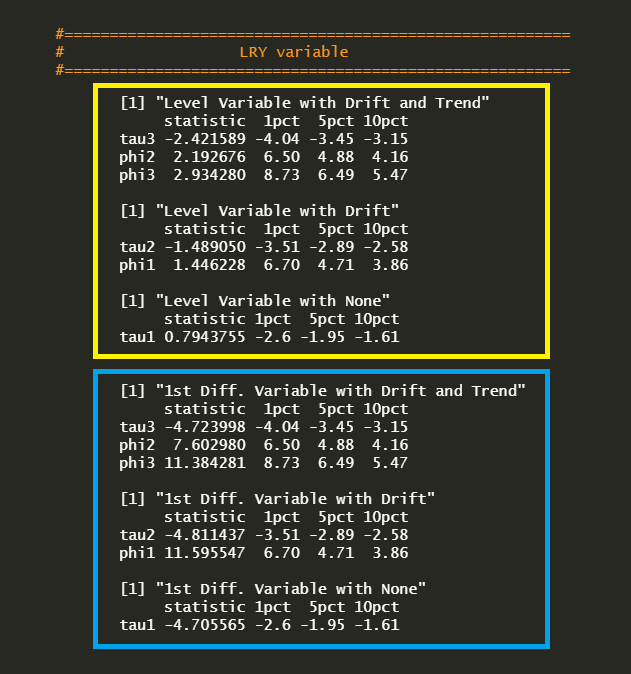
For the case of the LRY level variable (yellow box),

phi2 is insignificant : unit root(O), drift(X), trend(X)
phi3 is insignificant : unit root(O), drift(X)
tau3 is insignificant : unit root(O)

From the phi2(\(\phi2\))-statistic, joint null hypothesis is not rejected so that there is a unit root and we can exclude drift and trend terms. The phi3(\(\phi3\))-statistic shows that there is a unit root and we can exclude a drift term. Finally, the tau3(\(\tau3\))-statistic shows that there is a unit root.

The following test statistics are consistent with the above results and we can use a ADF test without a drift and trend terms.

phi1 is insignificant : unit root(O), drift(X)
tau2 is insignificant : unit root(O)

tau1 is insignificant : unit root(O)


For the case of the LRY 1st diff. variable (blue box), the same reasoning is used and we can find that there is no unit root but drift and trend terms are necessary.

phi2 is significant : unit root(X), drift(O), trend(O)
phi3 is significant : unit root(X), drift(O)
tau3 is significant : unit root(X)

phi1 is significant : unit root(X), drift(O)
tau2 is significant : unit root(X)

tau1 is significant : unit root(X)


Finally, we can conclude that logarithm of real income contains a unit root and can be stationay time series by differencing the first order. Now that this transformed variable contains no unit root, it can be included in VAR or VECM model.

In this process, the alphanumeric names of test statistics are a little confusing but when we refer the above three specifications of regression equations, the meanings of names of test statistics are clear.

Concluding Remarks

In this post, we’ve perform ADF test using R package and investigated the presence of a unit root by investigating several ADF test statistics. This is crucial to VAR model and in particular, VECM model.

Reference

Dickey, D. and W. Fuller (1979) Distribution of the Estimator for Autoregressive Time series with a Unit Root, Journal of the American Statistical Association 74, pp.427-431. \(\blacksquare\)