
Vector Autoregressive Model (VAR) using R
[This article was first published on K & L Fintech Modeling, and kindly contributed to R-bloggers]. (You can report issue about the content on this page here)
Want to share your content on R-bloggers? click here if you have a blog, or here if you don't.
This post gives a brief introduction to the estimation and forecasting of a Vector Autoregressive Model (VAR) model using R . We use vars and tsDyn R package and compare these two estimated coefficients. We also consider VAR in level and VAR in difference and compare these two forecasts.Want to share your content on R-bloggers? click here if you have a blog, or here if you don't.
VAR Model
VAR and VECM model
For a vector times series modeling, a vector autoregressive model (VAR) is used for describing the short-term dynamics. When there are the presence of long-term equilibrium relationships, a vector error correction model (VECM) is used, which consists of a VAR model and error correction equations.
In principle, there are three basic pairs of (model, data) in the context of the vector time series modeling. Given a vector of endogenous variables, \(X_t = (X_{1t}, X_{2t}, …, X_{kt})^{‘}\),
Firstly, when all variables are stationary in level (\(X_t\)), we use a VAR with stationary level variables (\(X_t\))
\[\begin{align} X_t = c + \beta_1 X_{t-1} +\beta_2 X_{t-2} + … + \epsilon_t \end{align}\]
Secondly, when all variables are non-stationary in level (\(X_t\)), we use a VAR with stationary growth variables (\(\Delta X_t\))
\[\begin{align} \Delta X_t = c + \beta_1 \Delta X_{t-1} +\beta_2 \Delta X_{t-2} + … + \epsilon_t \end{align}\]
Thirdly, when all variables are non-stationary in level (\(X_t\)) and there are some cointegrations in level(\(\Pi X_{t}\)), we use a VECM model which consists of a VAR with stationary growth variables (\(\Delta X_t\)) and error correcting equations with non-stationary level variables (\(X_t\)).
\[\begin{align} \Delta X_t = c + \beta_1 \Delta X_{t-1} +\beta_2 \Delta X_{t-2} + … + \Pi X_{t-1} + \epsilon_t \end{align}\]
Here, \(\Pi X_{t-1}\) is the first lag of linear combinations of non-stationary level variables or error correction terms (ECT) which represent long-term relationships among non-stationary level variables.
Since this post deals with VAR model, contents regarding stationarity and cointegration will be discussed in the next post.
For example, a tri-variate VAR(2) with differenced variables can be represented in the following way.
\[\begin{align} \begin{bmatrix} \Delta x_t \\ \Delta y_t \\ \Delta z_t \end{bmatrix} &=\begin{bmatrix} \gamma_{11}^1 & \gamma_{12}^1 & \gamma_{13}^1 \\ \gamma_{21}^1 & \gamma_{22}^1 & \gamma_{23}^1 \\ \gamma_{31}^1 & \gamma_{32}^1 & \gamma_{33}^1 \end{bmatrix} \begin{bmatrix} \Delta x_{t-1} \\ \Delta y_{t-1} \\ \Delta z_{t-1} \end{bmatrix} \\ &+\begin{bmatrix} \gamma_{11}^2 & \gamma_{12}^2 & \gamma_{13}^2 \\ \gamma_{21}^2 & \gamma_{22}^2 & \gamma_{23}^2 \\ \gamma_{31}^2 & \gamma_{32}^2 & \gamma_{33}^2 \end{bmatrix} \begin{bmatrix} \Delta x_{t-2} \\ \Delta y_{t-2} \\ \Delta z_{t-2} \end{bmatrix} \\ &+\begin{bmatrix} c_{11} & c_{12} \\ c_{21} & c_{22} \\ c_{31} & c_{32} \end{bmatrix} \begin{bmatrix} 1 \\ d_{t} \end{bmatrix} +\begin{bmatrix} \epsilon_{xt} \\ \epsilon_{yt} \\ \epsilon_{zt} \end{bmatrix} \end{align}\]
Lag Length p
Lag length (p) is selected by using several information criteria : AIC, HQ, SC, and so on. Lower these scores are better since these criteria penalize models that use more parameters. This work can be done easily by using VARselect() function with a maximum lag. From the following results, we set lag lengths of VAR in level and VAR in difference to 2 and 1 respectively.
1 2 3 4 5 6 7 8 9 10 11 12 13 14 | > VARselect(df.lev, lag.max = 4, + type = “const”, season = 4) $selection AIC(n) HQ(n) SC(n) FPE(n) 2 1 1 2 $criteria 1 2 3 4 AIC(n) -3.499648e+01 -3.515435e+01 -3.500078e+01 -3.486624e+01 HQ(n) -3.453329e+01 -3.445956e+01 -3.407440e+01 -3.370827e+01 SC(n) -3.378435e+01 -3.333616e+01 -3.257652e+01 -3.183593e+01 FPE(n) 6.393815e-16 5.601040e-16 6.876842e-16 8.607516e-16 | cs |
1 2 3 4 5 6 7 8 9 10 11 12 13 14 | > VARselect(df.diff, lag.max = 4, + type = “const”, season = 4) $selection AIC(n) HQ(n) SC(n) FPE(n) 1 1 1 1 $criteria 1 2 3 4 AIC(n) -3.476879e+01 -3.456481e+01 -3.418449e+01 -3.411838e+01 HQ(n) -3.430280e+01 -3.386583e+01 -3.325251e+01 -3.295340e+01 SC(n) -3.354510e+01 -3.272927e+01 -3.173710e+01 -3.105914e+01 FPE(n) 8.033856e-16 1.012233e-15 1.564343e-15 1.839676e-15 | cs |
Data
From urca R package, we can load denmark dataset which is used for estimating a money demand function of Denmark in Johansen and Juselius (1990). This dataset consists of logarithm of real money M2 (LRM), logarithm of real income (LRY), logarithm of price deflator (LPY), bond rate (IBO), bank deposit rate (IDE), which covers the period 1974:Q1 – 1987:Q3.

Visual inspections of this data in level show that real income rises, there is a demand for more money to make the transactions. On the other hand, the negative relationship between money and interest rate is found since the interest one gives up is the opportunity cost of holding money. It seems that there is a cointegration among money, income and interest rates.
In particular, when dealing with money demand function, it is important to include seasonal or monthly dummy variables to capture cyclical variations of money demand due simply to different seasonal and monthly patterns of payments or receipts.
R code
In principle, we need to check for the stationarity of each variables but in this exercise, we use both models of VAR in level and VAR in difference. It is because of the fact that many researchers usually use VAR model in difference but some researchers prefer to use VAR in level irrespective of the stationarity.
The following R code consists of 1) data loading, 2) VAR in level (vars package), 3) VAR in difference (vars package), and 4) VAR in difference (tsDyn package).
Since our model is a quarterly VAR for M2 demand, centered seasonal dummy variables are included as exogenous variables.
1 2 3 4 5 6 7 8 9 10 11 12 13 14 15 16 17 18 19 20 21 22 23 24 25 26 27 28 29 30 31 32 33 34 35 36 37 38 39 40 41 42 43 44 45 46 47 48 49 50 51 52 53 54 55 56 57 58 59 60 61 62 63 64 65 66 67 68 69 70 71 72 73 74 75 76 77 78 79 80 81 82 83 84 85 86 87 88 89 90 91 92 93 94 95 96 97 98 99 100 101 102 103 104 105 106 107 108 109 110 111 112 113 114 115 116 117 118 119 120 121 122 123 124 125 126 127 128 129 130 131 132 133 134 135 136 137 138 139 140 141 142 143 144 145 146 147 148 149 150 151 152 153 154 155 156 157 158 159 160 161 | #========================================================# # Quantitative ALM, Financial Econometrics & Derivatives # ML/DL using R, Python, Tensorflow by Sang-Heon Lee # # https://kiandlee.blogspot.com #——————————————————–# # Vector Autoregressive Model #========================================================# graphics.off() # clear all graphs rm(list = ls()) # remove all files from your workspace library(urca) # ca.jo, denmark library(vars) # vec2var #======================================================== # Data #======================================================== # forecasting horizon nhor <– 12 #——————————————– # quarterly data related with money demand #——————————————– # LRM : logarithm of real money M2 (LRM) # LRY : logarithm of real income (LRY) # LPY : logarithm of price deflator (LPY) # IBO : bond rate (IBO) # IDE : bank deposit rate (IDE) # the period 1974:Q1 – 1987:Q3 #——————————————– # selected variables data(denmark) df.lev <– denmark[,c(“LRM”,“LRY”,“IBO”,“IDE”)] m.lev <– as.matrix(df.lev) nr_lev <– nrow(df.lev) # quarterly centered dummy variables dum_season <– data.frame(yyyymm = denmark$ENTRY) substr.q <– as.numeric(substring(denmark$ENTRY, 6,7)) dum_season$Q2 <– (substr.q==2)–1/4 dum_season$Q3 <– (substr.q==3)–1/4 dum_season$Q4 <– (substr.q==4)–1/4 dum_season <– dum_season[,–1] # Draw Graph str.main <– c( “LRM=ln(real money M2)”, “LRY=ln(real income)”, “IBO=bond rate”, “IDE=bank deposit rate”) x11(width=12, height = 6); par(mfrow=c(2,2), mar=c(5,3,3,3)) for(i in 1:4) { matplot(m.lev[,i], axes=FALSE, type=c(“l”), col = c(“blue”), main = str.main[i]) axis(2) # show y axis # show x axis and replace it with # an user defined sting vector axis(1, at=seq_along(1:nrow(df.lev)), labels=denmark$ENTRY, las=2) } #======================================================== # VAR model in level #======================================================== # lag length VARselect(df.lev, lag.max = 4, type = “const”, season = 4) # estimation var.model_lev <– VAR(df.lev, p = 2, type = “const”, season = 4) # forecast of lev data var.pred <– predict(var.model_lev, n.ahead = nhor) x11(); par(mai=rep(0.4, 4)); plot(var.pred) x11(); par(mai=rep(0.4, 4)); fanchart(var.pred) #======================================================== # VAR model in difference using vars #======================================================== # 1st differenced data df.diff <– diff(as.matrix(df.lev), lag = 1) colnames(df.diff) <– c(“dLRM”, “dLRY”, “dIBO”, “dIDE”) m.diff <– as.matrix(df.diff) # lag length VARselect(df.diff, lag.max = 4, type = “const”, season = 4) # estimation vare_diff <– VAR(df.diff, p = 1, type = “const”, season = 4) # forecast of differenced data varf_diff <– predict(vare_diff, n.ahead = nhor) x11(); par(mai=rep(0.4,4)); plot(varf_diff) x11(); par(mai=rep(0.4,4)); fanchart(varf_diff) # recover lev forecast m.varf_lev_ft <– rbind(m.lev, matrix(NA, nhor, 4)) m.ft_df <– do.call(cbind,lapply(varf_diff$fcst, function(x) x[,“fcst”])) # growth to level for(h in (nr_lev+1):(nr_lev+nhor)) { hf <– h – nr_lev m.varf_lev_ft[h,] <– m.varf_lev_ft[h–1,] + m.ft_df[hf,] } # Draw Graph x11(width=8, height = 8); par(mfrow=c(4,1), mar=c(2,2,2,2)) for(i in 1:4) { df <– m.varf_lev_ft[,i] matplot(df, type=c(“l”), col = c(“blue”), main = str.main[i]) abline(v=nr_lev, col=“blue”) } #======================================================== # VAR model in difference using tsDyn #======================================================== linevare_diff <– lineVar(data = df.lev, lag = 1, include = “const”, model = “VAR”, I = “diff”, beta = NULL, exogen = dum_season) # check if both models (vars & tsDyn) yield same coefficients linevare_diff do.call(rbind,lapply(vare_diff$varresult, function(x) x$coefficients)) # quarterly centered dummy variables for forecast dumf_season <– rbind(tail(dum_season,4), tail(dum_season,4), tail(dum_season,4)) # forecast linevarf_diff <– predict(linevare_diff, n.ahead = nhor, exoPred = dumf_season) # Draw Graph x11(width=8, height = 8); par(mfrow=c(4,1), mar=c(2,2,2,2)) df <– rbind(df.lev, linevarf_diff) for(i in 1:4) { matplot(df[,i], type=c(“l”), col = c(“blue”), main = str.main[i]) abline(v=nr_lev, col=“blue”) } | cs |
In VAR in level, we can get the following forecasts by calling VAR() and predict() function.

In VAR in difference using vars R package, we can get the following forecasts by calling VAR() and predict() function.

In particular, VAR() model considers seasonal dummy variables automatically so that we don’t need to set seasonal dummy variables manually but have only to set season = 4.
However it does not produce level forecasts automatically when we use differenced data so that we need to convert the forecasts of differenced variables to the forecasts of level variables manually.
In VAR in difference using tsDyn R package, we can get the following forecasts by calling lineVar() and predict() function.

In particular, lineVar() model uses level variables and performs not VAR in level but VAR in difference by setting I = “diff”. It is convenient for us to get the forecasts of level variables not of differenced variables. There is no need for the conversion from differenced variables forecasts to level variables forecasts.
In VAR in difference using tsDyn R package, we can get the following forecasts by calling lineVar() and predict() function.
In particular, lineVar() model uses level variables and performs not VAR in level but VAR in difference by setting I = “diff”. It is convenient for us to get the forecasts of level variables not of differenced variables. There is no need for the conversion from differenced variables forecasts to level variables forecasts.
But unlike VAR() function, lineVar() function does not consider seasonal dummy variables automatically so that we need to set seasonal dummy variables manually by setting exogen = dum_season.
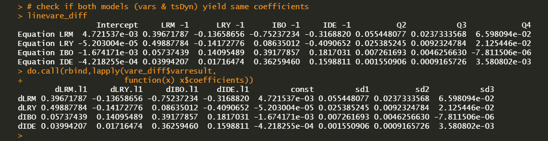
In the above R code, VAR() model and lineVar() model deal with the same representation. Therefore we can compare the estimated coefficients of these two models. From the output below, we can easily find that two estimated coefficients are the same.
In summary, we can figure out the differences of two forecasts. In other words, while VAR in level generated somewhat flattened forecasts, VAR in difference generated a little trended forecasts. These forecasts result from the assumption of underlying variables.
In this post, we’ve implemented R code for VAR estimation and forecasting. This is a reduced form model which is used for forecasting. Since our focus is on the level forecasts, we perform three works: 1) estimation and forecast of a VAR in level, 2) estimation of a VAR in difference and forecasts of level variables by using forecast of differenced variables, 3) estimation of a VAR in difference and forecasts of level variables directly. Next posts will cover the VECM model.
Johansen, S. and Juselius, K. (1990), Maximum Likelihood Estimation and Inference on Cointegration – with Applications to the Demand for Money, Oxford Bulletin of Economics and Statistics, 52, 2, 169–210. \(\blacksquare\)
In the above R code, VAR() model and lineVar() model deal with the same representation. Therefore we can compare the estimated coefficients of these two models. From the output below, we can easily find that two estimated coefficients are the same.
In summary, we can figure out the differences of two forecasts. In other words, while VAR in level generated somewhat flattened forecasts, VAR in difference generated a little trended forecasts. These forecasts result from the assumption of underlying variables.
Concluding Remarks
In this post, we’ve implemented R code for VAR estimation and forecasting. This is a reduced form model which is used for forecasting. Since our focus is on the level forecasts, we perform three works: 1) estimation and forecast of a VAR in level, 2) estimation of a VAR in difference and forecasts of level variables by using forecast of differenced variables, 3) estimation of a VAR in difference and forecasts of level variables directly. Next posts will cover the VECM model.
Reference
Johansen, S. and Juselius, K. (1990), Maximum Likelihood Estimation and Inference on Cointegration – with Applications to the Demand for Money, Oxford Bulletin of Economics and Statistics, 52, 2, 169–210. \(\blacksquare\)
To leave a comment for the author, please follow the link and comment on their blog: K & L Fintech Modeling.
R-bloggers.com offers daily e-mail updates about R news and tutorials about learning R and many other topics. Click here if you're looking to post or find an R/data-science job.
Want to share your content on R-bloggers? click here if you have a blog, or here if you don't.