Huge lines at gas stations have been seen around Turkey in recent days. Under the reason for this is the rise in the prices so often, in the last few months and the expectation to continue this. Of course, it is known that the rise in the exchange rate (US dollar to Turkish lira) has an important role in the hikes in gas prices. Considering the exchange currency crisis had been going on recently, it seems to be reasonable.

We will model the gas prices in terms of the exchange rate(xe), but this time, not only the current exchange rate but also, I want to add lagged values of xe to the model; Because the change of xe rates might not affect the prices immediately. Our model should be as below:

is ARIMA errors. is a lag level and can be determined by AICc.

The dataset we are going to use is that from 2019 to the present, gas prices and xe rates. In the code block below, we build tsibble data frame object and separate it into the train and test set.

library(tidyverse)
library(tidymodels)
library(readxl)
library(tsibble)
library(fable)
library(feasts)

df <- read_excel("gasoline.xlsx")

#Building tsibble dataset
df_tsbl <- df %>% 
  mutate(date=as.Date(date)) %>% 
  as_tsibble() %>%  
  fill_gaps() %>% #makes regular time series by filling the time gaps
  #fills in NAs with previous values
  fill(xe,gasoline,.direction = "down") 

#Separating into train and test set without random selection
#Takes first %75 for the training and the rest for the test set
df_split <- initial_time_split(df_tsbl, prop = 3/4)
df_train <- training(df_split)
df_test <- testing(df_split)

First of all, we will check the stationary of dependent and independent variables of the model as always.

#Checking the stationary
df_train %>% 
  pivot_longer(gasoline:xe) %>% 
  ggplot(aes(x=date,y=value))+
  geom_line()+
  facet_grid(vars(name),scales = "free_y")+
  xlab("")+ylab("")+
  theme_minimal()

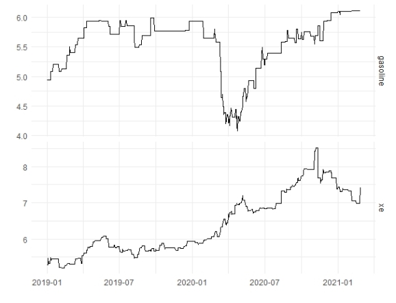
It seems that it is better we make differencing the gas and xe variables.

#Comparing the probable lagged models
model_lags_diff <- df_train %>% 
  #Excludes the first three days so all versions are in the same time period
  mutate(gasoline=c(NA,NA,NA,gasoline[4:788])) %>% 
  model(
    lag0 = ARIMA(gasoline ~ pdq(d = 1) + xe),
    lag1 = ARIMA(gasoline ~ pdq(d = 1) +
                   xe + lag(xe)),
    lag2 = ARIMA(gasoline ~ pdq(d = 1) +
                   xe + lag(xe) +
                   lag(xe, 2)),
    lag3 = ARIMA(gasoline ~ pdq(d = 1) +
                   xe + lag(xe) +
                   lag(xe, 2) + lag(xe, 3))
  )


glance(model_lags_diff) %>% 
  arrange(AICc) %>% 
  select(.model:AICc)

# A tibble: 4 x 5
# .model  sigma2 log_lik    AIC   AICc
#  <chr>    <dbl>   <dbl>  <dbl>  <dbl>
#1 lag1   0.00310   1152. -2294. -2294.
#2 lag2   0.00311   1152. -2292. -2292.
#3 lag3   0.00311   1152. -2290. -2290.
#4 lag0   0.00313   1148. -2288. -2288.

By the AICc results, it is better to select the one-level lagged model.

#Creates the model variable to the above results
model_lag1 <- df_train %>% 
  model(ARIMA(gasoline ~ pdq(d = 1) + xe + lag(xe)))


#Checking the model residuals consistency with white noise
model_lag1 %>% gg_tsresiduals()

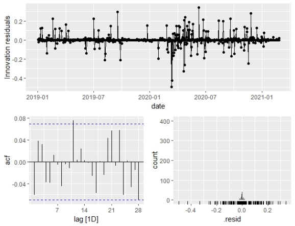
All the spikes seem to be within the threshold line to the ACF plot, so the residuals can be considered white noise. So, we are comfortable with the model we chose.

report(model_lag1)

#Series: gasoline 
#Model: LM w/ ARIMA(0,1,0)(2,0,0)[7] errors 

#Coefficients:
#        sar1    sar2       xe  lag(xe)
#      0.0920  0.1065  -0.0436   0.1060
#s.e.  0.0356  0.0359   0.0361   0.0368

#sigma^2 estimated as 0.003103:  log likelihood=1155.84
#AIC=-2301.69   AICc=-2301.61   BIC=-2278.35

The above results indicate that the model has the weekly seasonal AR(1) and AR(2) components. Now, we will predict with the test set by using the above regression equations to assess the accuracy of our model.

#Lagged Forecasts
model_pred <- forecast(model_lag1,df_test)

#Accuracy of the lagged model
cor(df_test$gasoline,model_pred$.mean) %>% round(2)

#[1] 0.77

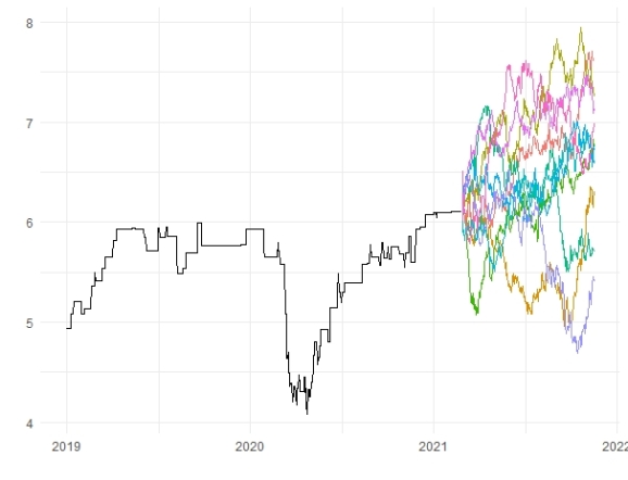
The result seems to be fine but we can try to improve it. In order to do that we will use bootstrapping and bagging methods.

set.seed(456)#getting the optimal and similar results for reproducibility 

#Bootstrapped forecasts
sim_fc <- model_lag1 %>% 
  fabletools::generate(new_data=df_test,
                       times=10,
                       bootstrap_block_size=14) %>% 
  select(-.model)


#Drawing bootstrapped forecasts
sim_fc %>% 
  autoplot(.sim)+
  autolayer(df_train,gasoline)+
  guides(color="none")+
  xlab("")+ylab("")+
  theme_minimal()

#Bagged forecasts
bagged_fc <- sim_fc %>% 
  summarise(bagged_mean=mean(.sim))

#Accuracy of bagging model  
cor(df_test$gasoline,bagged_fc$bagged_mean) %>% round(2)

#[1] 0.85

Quite a significant improvement for the accuracy of our model; it seems the bootstrapping simulation works in this process.