What is the Atkinson index?

The Atkinson index, introduced by Atkinson (1970) (Reference 1), is a measure of inequality used in economics. Given a population with values and an inequality-aversion parameter , the Atkinson index is defined as

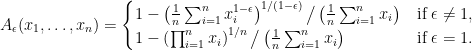
If we denote the Hölder mean by

then the Atkinson index is simply

While the index is defined for all , we restrict to be . (Some of the properties in the next section would not hold otherwise.)

Properties of the Atkinson index

The Atkinson index has a number of nice properties:

1. The index lies between 0 and 1, and is equal to 0 if and only if . Smaller values of the index indicate lower levels of inequality.
2. It satisfies the population replication axiom: If we replicate the population any number of times, the index remains the same.
3. It satisfies homogeneity: If we multiply by some positive constant , the index remains the same.
4. It satisfies the principle of transfers: If we transfer
5. It has only one parameter, , which represents the decision maker’s aversion to inequality. (See Section 2.3 of Reference 3 for one method of eliciting .)
6. It is computationally scalable: the sums in the numerator and denominator are amenable to the map-reduce paradigm, and so the index can be computed in a distributed fashion.

Some intuition for the Atkinson index

In R, the Atkinson function in the DescTools package implements the Atkinson index. It is so simple that I can reproduce the whole function here (most of the function is dedicated to checking for NA values):

function (x, n = rep(1, length(x)), parameter = 0.5, na.rm = FALSE) 
{
    x <- rep(x, n)
    if (na.rm) 
        x <- na.omit(x)
    if (any(is.na(x)) || any(x < 0)) 
        return(NA_real_)
    if (is.null(parameter)) 
        parameter <- 0.5
    if (parameter == 1) 
        A <- 1 - (exp(mean(log(x)))/mean(x))
    else {
        x <- (x/mean(x))^(1 - parameter)
        A <- 1 - mean(x)^(1/(1 - parameter))
    }
    A
}

To get some intuition for the Atkinson index, let’s look at the index for a population consisting of just 2 people. By homogeneity, we can assume that the first person has value 1; we will denote the second person’s value by x. We plot the Atkinson index for and , with ranging from to :

library(DescTools)

x <- 10^(-40:40 / 10)
eps <- 1
atkinsonIndex <- sapply(x,
  function(x) Atkinson(c(1, x), parameter = eps))

# log10 x axis
par(mfrow = c(1, 2))
plot(x, atkinsonIndex, type = "l", log = "x",
     ylab = "Atkinson index for (1, x)",
     main = "Atkinson index, eps = 1 (log x-axis)")

# regular x axis
plot(x, atkinsonIndex, type = "l", xlim = c(0, 1000),
     ylab = "Atkinson index for (1, x)",
     main = "Atkinson index, eps = 1 (linear x-axis)")

The two plots show the same curve, with the only difference being the x-axis (log scale on the left, linear scale on the right). The curve is symmetric around when the x-axis is on the log scale. We expect this since, by homogeneity, the index for is the same as the index for .

Next, we look at the Atkinson index for for a range of values for the parameter:

x <- 10^(0:40 / 10)
epsList <- 10^(-2:2 / 4)

plot(c(1, 10^4), c(0, 1), log = "x", type = "n",
     xlab = "x", ylab = "Atkinson index for (1, x)",
     main = "Atkinson index for various epsilon")
for (i in seq_along(epsList)) {
  atkinsonIndex <- sapply(x,
                          function(x) Atkinson(c(1, x), parameter = epsList[i]))
  lines(x, atkinsonIndex, col = i, lty = i, lwd = 2)
}
legend("topleft", legend = sprintf("%.2f", epsList), 
       col = seq_along(epsList), lty = seq_along(epsList), lwd = 2)

The larger is, the more “inequality-averse” we are. For fixed , the Atkinson index for increases as increases.

Finally, let’s look at what values the Atkinson index might take for samples taken from different distributions. In each of the panels below, we take 100 samples, each of size 1000. The samples are drawn from a log-t distribution with a given degrees of freedom (that is, the log of the values follows a t distribution). For each of these 100 samples, we compute the Atkinson index (with the default ), then make a histogram of the 100 index values. (The t distribution with is basically indistinguishable from the standard normal distribution.)

nsim <- 100
n <- 1000
dfList <- c(50, 10, 5, 3)

png("various-t-df.png", width = 900, height = 700, res = 120)
par(mfrow = c(2, 2))
set.seed(1)
for (dfVal in dfList) {
  atkinsonIndices <- replicate(nsim, Atkinson(exp(rt(n, df = dfVal))))
  hist(atkinsonIndices, xlim = c(0, 1),
       xlab = "Atkinson Index",
       main = paste("Histogram of Atkinson indices, df =", dfVal))
}
dev.off()

References:

1. Atkinson, A. B. (1970). On the Measurement of Inequality.
2. Wikipedia. Atkinson index.
3. Saint-Jacques, G., et. al. (2020). Fairness through Experimentation: Inequality in A/B testing as an approach to responsible design.