
Robustness Check for Maximum Smoothness Forward Rates using R
[This article was first published on K & L Fintech Modeling, and kindly contributed to R-bloggers]. (You can report issue about the content on this page here)
Want to share your content on R-bloggers? click here if you have a blog, or here if you don't.
This post makes a user-defined R function for Adams and Deventer (1994, revised 2010) maximum smoothness forward curve for the purpose of reusing and performs robustness checks for various initial term structures. We find that every time an initial term structure is changed, our procedure delivers correct output with different shapes of forward curves. Want to share your content on R-bloggers? click here if you have a blog, or here if you don't.
Maximum Smoothness Forward Rates
This post makes a R function for Adams-Deventer maximum smoothness forward curve based on previous post and performs robustness check for various initial term structures. Output of this post is the following figure describing various maximum smoothness forward rate curves with spot curves.

Details of maximum smoothness forward rate curve and its implementation are explained in the previous two posts below.
R user-defined function for Maximum Smoothness Forward Rates
For the purpose of reusing, previous post’s R code is structured as the next the user-defined R function. Here, we assume that a yield at time zero is the same as the yield at the shortest maturity.
1 2 3 4 5 6 7 8 9 10 11 12 13 14 15 16 17 18 19 20 21 22 23 24 25 26 27 28 29 30 31 32 33 34 35 36 37 38 39 40 41 42 43 44 45 46 47 48 49 50 51 52 53 54 55 56 57 58 59 60 61 62 63 64 65 66 67 68 69 70 71 72 73 74 75 76 77 78 79 80 81 82 83 84 85 86 87 88 89 90 91 92 93 94 95 96 97 98 99 100 101 102 103 104 105 106 107 108 109 110 111 112 113 114 115 116 117 118 119 120 121 122 123 124 125 126 127 128 129 130 131 132 133 134 135 136 137 138 139 140 141 142 143 144 145 146 147 148 149 150 151 152 153 154 155 156 157 158 159 160 161 162 163 164 165 166 167 168 169 170 171 172 173 174 175 176 177 178 179 180 181 182 183 184 185 186 187 188 189 190 191 192 193 194 195 | #========================================================# # Quantitative ALM, Financial Econometrics & Derivatives # ML/DL using R, Python, Tensorflow by Sang-Heon Lee # # https://kiandlee.blogspot.com #——————————————————–# # Adams and Deventer Maximum Smoothness Forward Curve # Robustness Check using a user-defined function #========================================================# graphics.off() # clear all graphs rm(list = ls()) # remove all files from your workspace # function for Maximum Smoothness Forward Curve func_msfc <– function(df.mkt) { # maturity strings for figure v.str.mat <– paste0(as.character(df.mkt$mat), “Y”) # number of maturity n <– length(df.mkt$mat) # add 0-maturity zero rate (assumption) df <– rbind(c(0, df.mkt$zrc[1]), df.mkt) #df <- rbind(c(0, 0.04), df.mkt) # discount factor df$DF <– with(df, exp(–zrc*mat)) # -ln(P(t(i)/t(i-1))) df$mln <– c(NA,–log(df$DF[1:n+1]/df$DF[1:n])) # ti^n df$t5 <– df$mat^5 df$t4 <– df$mat^4 df$t3 <– df$mat^3 df$t2 <– df$mat^2 df$t1 <– df$mat^1 df$t0 <– 1 # dti = ti^n-(ti-1)^n df$dt5 <– c(NA,df$t5[1:n+1] – df$t5[1:n]) df$dt4 <– c(NA,df$t4[1:n+1] – df$t4[1:n]) df$dt3 <– c(NA,df$t3[1:n+1] – df$t3[1:n]) df$dt2 <– c(NA,df$t2[1:n+1] – df$t2[1:n]) df$dt1 <– c(NA,df$t1[1:n+1] – df$t1[1:n]) #———————————————— # construction linear system #———————————————— mQ <– mA <– matrix(0, nrow = 5*n, ncol = 5*n) vC <– vB <– rep(0,5*n) # Objective function for(r in 1:n) { mQ[((r–1)*5+1):((r–1)*5+3),((r–1)*5+1):((r–1)*5+3)] <– matrix(with(df[r+1,], c(144/5*dt5, 18*dt4, 8*dt3, 18*dt4, 12*dt3, 6*dt2, 8*dt3, 6*dt2, 4*dt1)),3,3) } # Smoothness Constraints : f, f’, f”, f”’ for (r in 1:4) { for(t in 1:(n–1)) { if(r==1) { temp <– with(df[t+1,], c(t4, t3, t2, t1, t0)) } else if(r==2) { temp <– with(df[t+1,], c(4*t3, 3*t2, 2*t1, t0)) } else if(r==3) { temp <– with(df[t+1,], c(12*t2, 6*t1, 2*t0)) } else if(r==4) { temp <– with(df[t+1,], c(24*t1, 6*t0)) } mA[(r–1)*(n–1)+t,((t–1)*5+1):((t–1)*5+6–r)] <– temp mA[(r–1)*(n–1)+t,((t–0)*5+1):((t–0)*5+6–r)] <– –temp } } # bond price fitting constraints r = 5; for(t in 1:n) { temp <– with(df[t+1,], c(dt5/5,dt4/4,dt3/3,dt2/2,dt1)) mA[(r–1)*(n–1)+t,((t–1)*5+1):((t–0)*5)] <– temp } # additional four constraints r = 5*n–3; c = 5 ; mA[r,c] <– 1 r = 5*n–2; c = 5–1; mA[r,c] <– 1 r = 5*n–1; c = (5*(n–1)+1):(5*(n–1)+4) mA[r,c] <– with(df[n+1,], c(4*t3, 3*t2, 2*t1, t0)) r = 5*n–0; c = (5*(n–1)+1):(5*(n–1)+3) mA[r,c] <– with(df[n+1,], c(12*t2, 6*t1, 2*t0)) # RHS vector vC <– rep(0,5*n) vB <– c(rep(0,4*(n–1)), df$mln[2:(n+1)], df$zrc[1],0,0,0) # concatenation of matrix and vector AA = rbind(cbind(mQ, –t(mA)), cbind(mA, matrix(0,5*n,5*n))) BB = c(–vC, vB) #———————————————— # solve linear system by using inverse matrix #———————————————— XX = solve(AA)%*%BB XX # save and print calibrated parameters for(i in 1:n) { df.mkt[i,c(“a”,“b”,“c”,“d”,“e”)] <– XX[((i–1)*5+1):(i*5)] } df.coef <– df.mkt[,c(“a”,“b”,“c”,“d”,“e”)] #———————————————— # monthly forward rate and spot rate #———————————————— df.mm <– data.frame( mat = seq(0,10,1/12),y = NA, fwd = NA) # which segment df.mm$seg_no <– apply(df.mm, 1, function(x) min(which(x[1]<=df.mkt$mat)) ) # ti^n df.mm$t5 <– df.mm$mat^5 df.mm$t4 <– df.mm$mat^4 df.mm$t3 <– df.mm$mat^3 df.mm$t2 <– df.mm$mat^2 df.mm$t1 <– df.mm$mat^1 df.mm$t0 <– 1 nr <– nrow(df.mm) # number of rows # dti = ti^n-(ti-1)^n df.mm$dt5 <– c(NA,df.mm$t5[2:nr] – df.mm$t5[1:(nr–1)]) df.mm$dt4 <– c(NA,df.mm$t4[2:nr] – df.mm$t4[1:(nr–1)]) df.mm$dt3 <– c(NA,df.mm$t3[2:nr] – df.mm$t3[1:(nr–1)]) df.mm$dt2 <– c(NA,df.mm$t2[2:nr] – df.mm$t2[1:(nr–1)]) df.mm$dt1 <– c(NA,df.mm$t1[2:nr] – df.mm$t1[1:(nr–1)]) # monthly maximum smoothness forward curve df.mm$fwd[1] <– df.mkt$e[1] # time 0 forward rate df.mm$y[1] <– df.mkt$e[1] # time 0 yield temp_y_sum <– 0 for(i in 2:nr) { mat <– df.mm$mat[i] seg_no <– df.mm$seg_no[i] # which segment v_tn <– df.mm[i,c(“t4”,“t3”,“t2”,“t1”,“t0”)] v_dtn <– df.mm[i,c(“dt5”,“dt4”,“dt3”,“dt2”,“dt1”)] v_abcde <– df.mkt[seg_no, c(“a”,“b”,“c”,“d”,“e”)] # monthly maximum smoothness forward curve df.mm$fwd[i] <– sum(v_abcde*v_tn) # monthly yield curve temp_y_sum <– temp_y_sum + sum(c(1/5,1/4,1/3,1/2,1)*v_abcde*v_dtn) df.mm$y[i] <– (1/mat)*temp_y_sum } #———————————————— # Draw Graph #———————————————— x11(width=8, height = 6); plot(df.mkt$mat, df.mkt$zrc, col = “red”, cex = 1.5, ylim = c(min(df.mm$fwd)–0.01,max(df.mm$fwd)+0.01), xlab = “Maturity”, ylab = “Interest Rate”, lwd = 10, main = “Monthly Maximum Smoothness Forward Rates and Spot Rates”) text(df.mkt$mat, df.mkt$zrc+(max(df.mm$fwd)–min(df.mm$fwd))/12, labels=v.str.mat, cex= 1.5) lines(df.mm$mat, df.mm$y , col = “blue” , lwd = 5) lines(df.mm$mat, df.mm$fwd, col = “green”, lwd = 10) legend(“bottomright”, legend=c(“Spot Curve”,“Forward Curve”,“Input Spot Rates”), col=c(“blue”,“green”,“red”), pch = c(15,15,16), border=“white”, box.lty=0, cex=1.5) XX2 <– solve(mA)%*%vB cbind(XX[1🙁5*n)],XX2,XX[1🙁5*n)]–XX2) sum(abs(XX[1🙁5*n)]–XX2)) return(list(mm=df.mm, coef = df.coef)) } | cs |
Robustness Check
For robustness check, we change a initial term structure a little and draw graph and print coefficients. Since we made a user-defined R code, this job can be done simply by using the following R code.
1 2 3 4 5 6 7 8 9 10 11 12 13 14 15 16 17 18 19 20 21 22 23 24 | #———————————————— # Robustness Check #———————————————— # Input : market zero rate, maturity df.mkt <– data.frame( mat = c(0.25, 1, 3, 5, 10), zrc = c(4.75, 4.5, 5.5, 5.25, 6.5)/100) lt1 <– func_msfc(df.mkt); lt1$coef df.mkt <– data.frame( mat = c(0.25, 1, 3, 5, 7, 10), zrc = c(4.75, 4.5, 5.5, 5.25, 7, 6.5)/100) lt2 <– func_msfc(df.mkt); lt2$coef df.mkt <– data.frame( mat = c(0.25, 1, 3, 5, 7, 8, 10), zrc = c(4.75, 4.5, 5.5, 5.25, 7, 4, 6.5)/100) lt3 <– func_msfc(df.mkt); lt3$coef df.mkt <– data.frame( mat = c(0.25, 1, 3, 4, 5, 7, 8, 10), zrc = c(4.75, 4.5, 5.5, 8, 5.25, 7, 4, 6.5)/100) lt4 <– func_msfc(df.mkt); lt4$coef | cs |
Running the above R code for robustness check, we can get the following table of coefficients. As the number of maturity of a initial term structure increases, the number of parameters increases in multiples of 5.
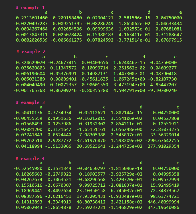
With these estimated coefficients, we can draw the following maximum smoothness forward (green solid line) and spot (blue solid line) curve with each initial term structure (red dot point).
Concluding Remarks
So far through three posts regarding Adams-Deventer maximum smoothness forward curve, we can understand and implement this powerful model. In particular, we make a user-defined R function for another usages. \(\blacksquare\)
To leave a comment for the author, please follow the link and comment on their blog: K & L Fintech Modeling.
R-bloggers.com offers daily e-mail updates about R news and tutorials about learning R and many other topics. Click here if you're looking to post or find an R/data-science job.
Want to share your content on R-bloggers? click here if you have a blog, or here if you don't.