
Adams and Deventer Maximum Smoothness Forward Rate Curve using R code
[This article was first published on K & L Fintech Modeling, and kindly contributed to R-bloggers]. (You can report issue about the content on this page here)
Want to share your content on R-bloggers? click here if you have a blog, or here if you don't.
This post implements Adams and Deventer (1994) approach which generates the best fitting yield curve smoothing with the principle of maximum smoothness forward rate curve. This provides a powerful closed-form solution by which we can sidestep a kinked or zigzag problem of forward rate curve effectively. Want to share your content on R-bloggers? click here if you have a blog, or here if you don't.
Computing Maximum Smoothness Forward Rate Curve
To ensure a smoothness of the yield curve, the Adam-Deventer method can be used.
- Adams K.J. and D. R. van Deventer (1994), Fitting yield curves and forward rate curves with maximum smoothness, Journal of Fixed Income 4-1, pp. 52-62.
- Imai K. and D. R. van Deventer (1996), Financial Risk Analytics Book
- van Deventer, D. R. (2010), Basic Building Blocks of Yield Curve Smoothing, Part 10: Maximum Smoothness Forward Rates and Related Yields versus Nelson-Siegel (Revised May 8, 2012)
- Lim, K. G. and Q. Xiao (2002), Computing maximum smoothness forward rate curves, Statistics and Computing 12, pp. 275-279.
We use the Deventer (2010) revised methodology, from which we borrow input data also as follows.
1 2 3 4 5 6 7 8 9 10 11 12 13 | —————————————— Maturity Spot Rate ZCB Price —————————————— t r P(0,t) —————————————— 0.25 4.75% 0.9882 1 4.50% 0.9560 3 5.50% 0.8479 5 5.25% 0.7691 10 6.50% 0.5220 —————————————— | cs |
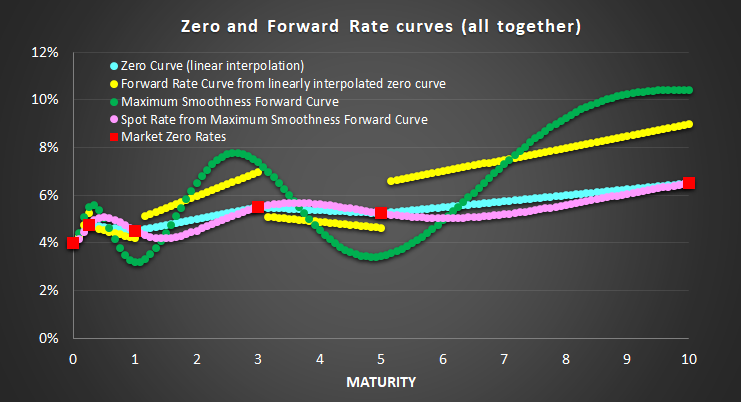
Using a linear interpolation of the given market zero curve, we can calculate next monthly zero curve and forward curve. As can be seen in figure below, forward rate from linearly interpolated show discontinuity and no smoothness (some forward rates are omitted because they show too large deviations as outliers).

To ensure a smooth yield curve, Adams and Deventer (1994) use maximum smoothness forward rate approach. Their approach delivers a smooth yield curve like the following figure.
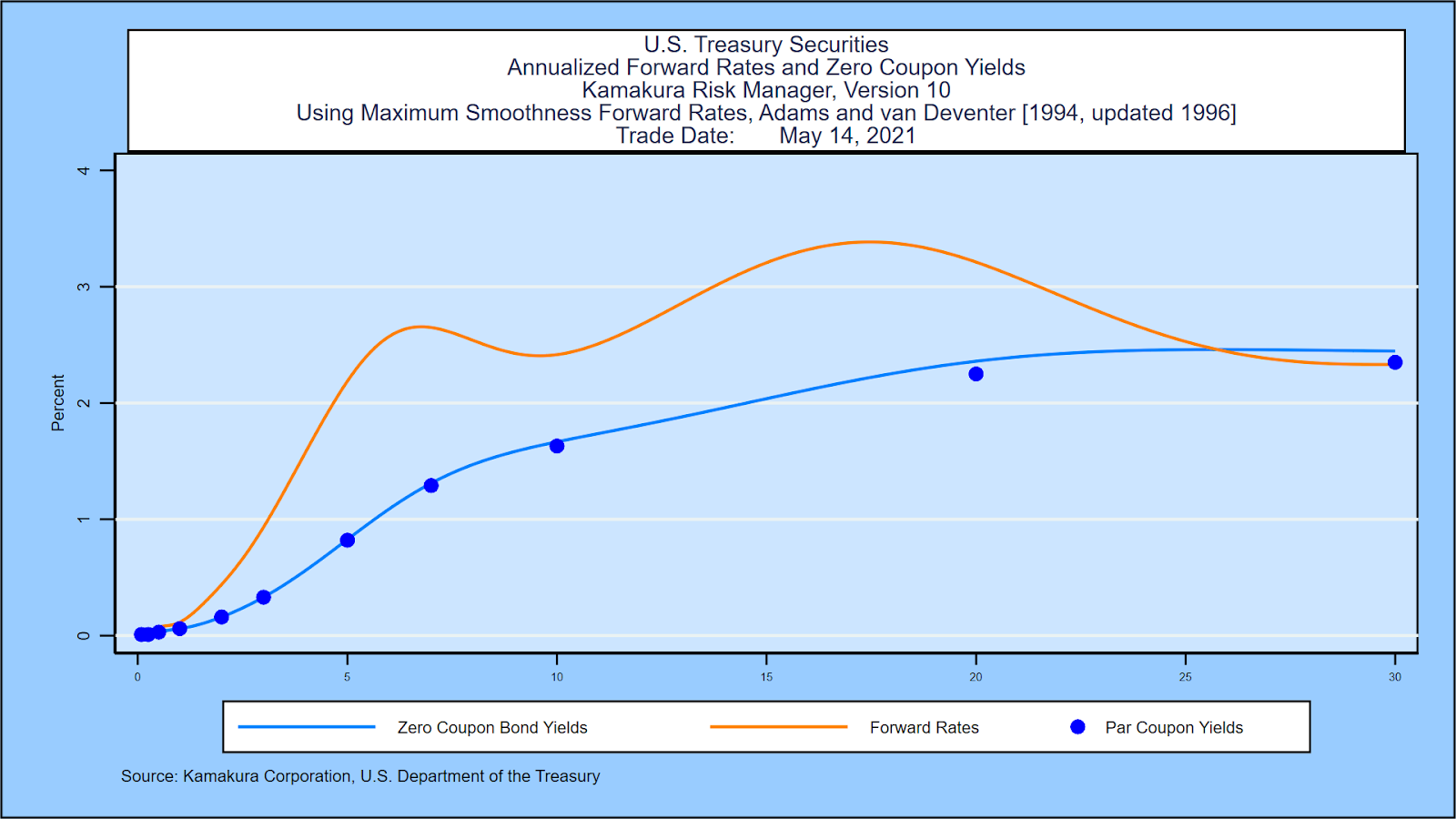 source : Kamakura Corporation
 Forward Rate
To evaluate smoothness numerically, Adams and Deventer (1994) calculate the second derivative of forward rate for each segments (intervals between observed maturities), the squared sum of them, and minimize this with some constraints which ensure smoothness of yield curve.
In each forward rate curve segment, each forward rate \(f(t)\) is assumed to have the following form.
\[\begin{align} f(t) &= a_i t^4 + b_i t^3 + c_i t^2 + d_i t + e_i \\ \\ &t_{i-1} \lt t \le t_{i}, \quad i=1,2,…,m \end{align}\]
The subscript i denotes the segment number. In case of the example data, as the number of coefficients are \(25 = 5 \times 5\), it is desirable to construct 25 constraints.
Objective Function
The i-th objective function maximizes a smoothness of forward rates, which is an integration of twice differenced forward rates. \[\begin{align} \int_{t_{i-1}}^{t_i} [f^{”}(t)]^2 dt &= \int_{t_{i-1}}^{t_i} \left[12a_i t^2 + 6 b_i t + 2 c_i \right]^2 dt \\ &= \frac{144}{5} \Delta t_i^5 a_i^2 + 36 \Delta t_i^4 a_i b_i + 12 \Delta t_i^3 b_i^2 \\ &+ 16 \Delta t_i^3 a_i c_i + 12 \Delta t_i^2 b_i c_i + 4 \Delta t_i c_i^2 \end{align}\]
Equality Linear Constraints
For \(i=1,2,…,m-1 \), restrictions on continuity of \(f\), \(f^{‘}\),\(f^{”}\) and \(f^{”’}\) are imposed.
\[\begin{align} &a_{i+1} t^4 + b_{i+1} t^3 + c_{i+1} t^2 + d_{i+1} t + e_{i+1} \\ &= a_i t^4 + b_i t^3 + c_i t^2 + d_i t + e_i \\ \\ & 4a_{i+1} t^3 + 3b_{i+1} t^2 + 2c_{i+1} t + d_{i+1} \\ &= 4a_i t^3 + 3b_i t^2 + 2c_i t + d_i\\ \\ &12a_{i+1} t^2 + 6b_{i+1} t + 2c_{i+1} = 12a_{i} t^2 + 6b_{i} t + 2c_{i} \\ \\ & 24 a_{i+1} t + 6b_{i+1} = 24a_{i} t + 6 b_{i} \end{align}\]
For \(i=1,2,…,m \), a set of integration of forward rates should fit a set of zero coupon bond price.
\[\begin{align} -log\left[ \frac{P_i}{P_{i-1}}\right] &= \frac{1}{5} a_i (t_i^5 – t_{i-1}^5) + \frac{1}{4} b_i (t_i^4 – t_{i-1}^4) \\ &+ \frac{1}{3} c_i (t_i^3 – t_{i-1}^3) + \frac{1}{2} d_i (t_i^2 – t_{i-1}^2) + e_i (t_i – t_{i-1}) \end{align}\]
These restrictions can be rewritten more compactly (\(\Delta k_{i+1}= k_{i+1} – k_{i}, \Delta t_i^n= t_i^n – t_{i-1}^n\)). \[\begin{align} 0 &= \Delta a_{i+1} t^4 + \Delta b_{i+1} t^3 + \Delta c_{i+1} t^2 + \Delta d_{i+1} t + \Delta e_{i+1} \\ 0 &= 4\Delta a_{i+1} t^3 + 3\Delta b_{i+1} t^2 + 2\Delta c_{i+1} t + d\Delta _{i+1} \\ 0 &= 12\Delta a_{i+1} t^2 + 6\Delta b_{i+1} t + 2\Delta c_{i+1} \\ 0 &= 24\Delta a_{i+1} t + 6\Delta b_{i+1} \end{align}\] \[\begin{align} -log\left[ \frac{P_i}{P_{i-1}}\right] = \frac{1}{5} a_i \Delta t_i^5 + \frac{1}{4} b_i \Delta t_i^4 + \frac{1}{3} c_i \Delta t_i^3 + \frac{1}{2} d_i \Delta t_i^2 + e_i \Delta t_i \end{align}\]
From these, we have \(21 = 4 \times 4 + 5\) constraints and additional 4 constraints are required.
Additional Constraints
The initial forward rate is assumed to be equal to the observed spot rate or given other rate at time zero. Three remaining constraints are related to the smoothness of forward rate at time 0 and T using the first or second derivative of forward rate.
\[\begin{align} f(0) = r(0) \\ f^{‘}(0) = 0 \\ f^{‘}(T) = 0 \\ f^{”}(T) = 0 \end{align}\]
Now we have a problem of 25 unknowns and 25 equations.
R code
We use optimization to solve for this 25 unknown variables problem using NlcOptim R package which have two main arguments : 1) objective function and 2) constraints function. In particular, constraints function can deal with both linear and non-linear constraints. The following R code estimate 25 coefficients of Adams-Deventer’s maximum smoothness forward rate curve.
1 2 3 4 5 6 7 8 9 10 11 12 13 14 15 16 17 18 19 20 21 22 23 24 25 26 27 28 29 30 31 32 33 34 35 36 37 38 39 40 41 42 43 44 45 46 47 48 49 50 51 52 53 54 55 56 57 58 59 60 61 62 63 64 65 66 67 68 69 70 71 72 73 74 75 76 77 78 79 80 81 82 83 84 85 86 87 88 89 90 91 92 93 94 95 96 97 98 99 100 101 102 103 104 105 106 107 108 109 110 111 112 113 114 115 116 117 118 119 120 121 122 123 124 125 126 127 128 129 130 131 132 133 134 | #========================================================# # Quantitative ALM, Financial Econometrics & Derivatives # ML/DL using R, Python, Tensorflow by Sang-Heon Lee # # https://kiandlee.blogspot.com #——————————————————–# # Adams and Deventer Maximum Smoothness Forward Curve # using non-linear optimization #========================================================# graphics.off() # clear all graphs rm(list = ls()) # remove all files from your workspace library(NlcOptim) # optimization with non-linear constraints # whole calculation process f_calc <– function(x0) { # number of maturity n <– length(df.mkt$mat) # add 0-maturity zero rate (assumption) #df <- rbind(c(0, df.mkt$zrc[1]), df.mkt) df <– rbind(c(0, 0.04), df.mkt) # discount factor df$DF <– with(df, exp(–zrc*mat)) # -ln(P(t(i)/t(i-1))) df$mln <– c(NA,–log(df$DF[1:n+1]/df$DF[1:n])) # ti^n df$t5 <– df$mat^5 df$t4 <– df$mat^4 df$t3 <– df$mat^3 df$t2 <– df$mat^2 df$t1 <– df$mat^1 # dti = ti^n-(ti-1)^n df$dt5 <– c(NA,df$t5[1:n+1] – df$t5[1:n]) df$dt4 <– c(NA,df$t4[1:n+1] – df$t4[1:n]) df$dt3 <– c(NA,df$t3[1:n+1] – df$t3[1:n]) df$dt2 <– c(NA,df$t2[1:n+1] – df$t2[1:n]) df$dt1 <– c(NA,df$t1[1:n+1] – df$t1[1:n]) # parameters to be found df$e <– df$d <– df$c <– df$b <– df$a <– c(NA,rep(0,n)) df$a[1:n+1] <– x0[(0*n+1):(1*n)] df$b[1:n+1] <– x0[(1*n+1):(2*n)] df$c[1:n+1] <– x0[(2*n+1):(3*n)] df$d[1:n+1] <– x0[(3*n+1):(4*n)] df$e[1:n+1] <– x0[(4*n+1):(5*n)] # difference of coefficients : dki = ki – k(i-1) df$da <– c(NA, df$a[2:n] – df$a[2:n+1], NA) df$db <– c(NA, df$b[2:n] – df$b[2:n+1], NA) df$dc <– c(NA, df$c[2:n] – df$c[2:n+1], NA) df$dd <– c(NA, df$d[2:n] – df$d[2:n+1], NA) df$de <– c(NA, df$e[2:n] – df$e[2:n+1], NA) # forward rate df$fwd <– NA df$fwd[1:n+1] <– with(df[1:n+1,], a*t4 + b*t3 + c*t2 +d*t1 + e) df$fwd[1] <– df$e[2] # linear constraints df$cmln <– df$cfp3 <– df$cfp2 <– df$cfp1<– df$cfp0<– NA df$cfp0[2:n] <– with(df[2:n,], da*t4 + db*t3 + dc*t2 + dd*t1 + de) df$cfp1[2:n] <– with(df[2:n,], 4*da*t3 + 3*db*t2 + 2*dc*t1 + dd) df$cfp2[2:n] <– with(df[2:n,], 12*da*t2 + 6*db*t1 + 2*dc) df$cfp3[2:n] <– with(df[2:n,], 24*da*t1 + 6*db) df$cmln[2:(n+1)] <– with(df[2:(n+1),], a*dt5/5 + b*dt4/4 + c*dt3/3 + d*dt2/2 + e*dt1 – mln) # additional 4 constraint # initial(0) forward rate(f) = r0, initial f’ = 0 # terminal(T) f’, f” = 0 const_f_0 <– df$e[2] – df$zrc[1] const_f1_0 <– df$d[2] const_f1_T <– with(df[n+1,], 4*a*t3 + 3*b*t2 + 2*c*t1 + d) const_f2_T <– with(df[n+1,], 12*a*t2 + 6*b*t1 + 2*c) # objective function df$obj <– NA df$obj[1:n+1] <– with(df[1:n+1,], (144/5)*dt5*a^2 + 36*dt4*a*b + 12*dt3*b^2 + 16*dt3*a*c + 12*dt2*b*c + 4*dt1*c^2) return(list(df.calc = df, fvalue = sum(df$obj[1:n+1]), const = c( df$cfp0[2:n], df$cfp1[2:n], df$cfp2[2:n], df$cfp3[2:n], df$cmln[2:(n+1)], const_f_0, const_f1_0, const_f1_T, const_f2_T))) } # objective function for solnl obj <– function(x) { lt.out <– f_calc(x); return(lt.out$fvalue) } # constraint function for solnl con <– function(x) { lt.out <– f_calc(x) return(list(ceq = lt.out$const, c = NULL)) } # Input : market zero rate, maturity df.mkt <– data.frame( mat = c(0.25, 1, 3, 5, 10), zrc = c(4.75, 4.5, 5.5, 5.25, 6.5)/100 ) x0 <– rep(0.001,25) # initial guesses out <– solnl(x0, objfun = obj, confun = con) # augment df.mkt with calibrated paramters n <– length(df.mkt$mat) df.mkt$a[1:n] <– out$par[(0*n+1):(1*n)] df.mkt$b[1:n] <– out$par[(1*n+1):(2*n)] df.mkt$c[1:n] <– out$par[(2*n+1):(3*n)] df.mkt$d[1:n] <– out$par[(3*n+1):(4*n)] df.mkt$e[1:n] <– out$par[(4*n+1):(5*n)] df.mkt | cs |
Running the above R code, we can obtain calibrated parameters (\(a_i, b_i, c_i, d_i, e_i\), \(i=1,…,m \)) which characterize the maximum smoothness forward curve.
It is typical to set the time 0 spot rate to the shortest term rate but Deventer (2010) use 4% and we follow this setting.
1 2 3 4 5 6 7 | mat zrc a b c d e 1 0.25 0.0475 3.7020078185 -3.343981375 0.8481712 1.429488e-16 0.04000000 2 1.00 0.0450 -0.1354629771 0.493489420 -0.5908803 2.398419e-01 0.02500988 3 3.00 0.0550 0.0080049880 -0.080382440 0.2699275 -3.340299e-01 0.16847782 4 5.00 0.0525 -0.0024497294 0.045074169 -0.2946273 7.950796e-01 -0.67835429 5 10.00 0.0650 0.0002985362 -0.009891143 0.1176126 -5.790532e-01 1.03931172 | cs |
Substituting these calibrated parameters into the above equations for forward rate and yield curve, we can draw the next figure. Green line is the maximum smoothness forward rate. we can easily find that this forward rate is continuous and very smooth unlike the forward rate from the linearly interpolated zero rate (yellow line).
Concluding Remarks
From this post, we have implemented Adams and Deventer’s maximum smoothness forward rate curve. This is a powerful approach for fitting yield curve. But in principle, this problem is solved by closed form solution because it is a quadratic optimization with equality linear constraints. This topic will be covered in the next post. \(\blacksquare\)
To leave a comment for the author, please follow the link and comment on their blog: K & L Fintech Modeling.
R-bloggers.com offers daily e-mail updates about R news and tutorials about learning R and many other topics. Click here if you're looking to post or find an R/data-science job.
Want to share your content on R-bloggers? click here if you have a blog, or here if you don't.