The Turkish president thinks that high interest rates cause inflation, contrary to the traditional economic approach. For this reason, he dismissed two central bank chiefs within a year. And yes, unfortunately, the central bank officials have limited independence doing their job in Turkey contrary to the rest of the world.

In order to check that we have to model inflation rates with some variables. The most common view of the economic authorities is that the variables affecting the rates are currency exchange rates, and CDS(credit default swap). Of course, we will also add the funding rates variable, the president mentioned, to the model to compare with the other explanatory variables.

Because the variables can be highly correlated with each other, we will prefer the random forest model. This algorithm also has a built-in function to compute the feature importance.

Random Forest; for regression, constructs multiple decision trees and, inferring the average estimation result of each decision tree. This algorithm is more robust to overfitting than the classical decision trees.

The random forest algorithms average these results; that is, it reduces the variation by training the different parts of the train set. This increases the performance of the final model, although this situation creates a small increase in bias.

The random forest uses bootstrap aggregating(bagging) algortihms. We would take for training sample, X = x₁, …, x_n and, Y = y₁, …, y_n for the outputs. The bagging process repeated B times with selecting a random sample by changing the training set and, tries to fit the relevant tree algorithms to the samples. This fitting function is denoted f_b in the below formula.

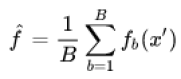
The unseen values, x’, would be fitted by f_b and then all the results of B individuals trees are averaged. Random forest selects explanatory variables at each variable split in the learning process, which means it trains a random subset of the feature instead of all sets of features. This is called feature bagging. This process reduces the correlation between trees; because the strong predictors could be selected by many of the trees, and it could make them correlated.

The permutation feature importance method would be used to determine the effects of the variables in the random forest model. This method calculates the increase in the prediction error(MSE) after permuting the feature values. If the permuting wouldn’t change the model error, the related feature is considered unimportant. We will use the varImp function to calculate variable importance. It has a default parameter, scale=TRUE, which scales the measures of importance up to 100.

The data we are going to use can be download here. The variables we will examine:

• cpi: The annual consumer price index. It is also called the inflation rate. This is our target variable.
• funding_rate: The one-week repo rate, which determined by the Turkish Central Bank. It is also called the political rate.
• exchange_rate: The currency exchange rates between Turkish Liras and American dollars.
• CDS: The credit defaults swap. It kind of measures the investment risk of a country or company. It is mostly affected by foreign policy developments in Turkey. Although the most popular CDS is 5year, I will take CDS of 1 year USD in this article.

library(readxl)
library(dplyr)
library(ggplot2)
library(randomForest)
library(varImp)

#Create the dataframe
df <- read_excel("cpi.xlsx")

#Random Forest Modelling
model <- randomForest(CPI ~ funding_rate+exchange_rate, 
                          data = df, importance=TRUE) 

#Conditional=True, adjusts for correlations between predictors.
i_scores <- varImp(model, conditional=TRUE)

#Gathering rownames in 'var'  and converting it to the factor
#to provide 'fill' parameter for the bar chart. 
i_scores <- i_scores %>% tibble::rownames_to_column("var") 
i_scores$var<- i_scores$var %>% as.factor()

#Plotting the bar and polar charts for comparing variables
i_bar <- ggplot(data = i_scores) + 
  geom_bar(
    stat = "identity",#it leaves the data without count and bin
    mapping = aes(x = var, y=Overall, fill = var), 
    show.legend = FALSE,
    width = 1
  ) + 
  labs(x = NULL, y = NULL)

i_bar + coord_polar() + theme_minimal()
i_bar + coord_flip() + theme_minimal()

When we examine the charts above, we can clearly see that the funding and exchange rates have similar effects on the model and, CDS has significant importance in the behavior of the CPI. So the theory of the president seems to fall short of what he claims.

References

• Wikipedia: Random Forest
• Interpretable Machine Learning: Permutation Feature Importance
• The Caret Package: The Variable Importance
• R for Data Science: Coordinate systems
• How to Find the Most Important Variables in R