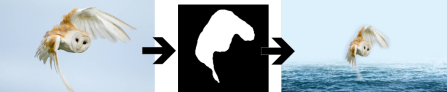
Today we want to train a deep learning model that detects a foreground object on an image (say, a bird), automatically crops the bird and removes the background, and pastes the bird onto a new background.

So we want to automate this process:

Why would you want to do this?

A number of applications come to mind. For instance, if you have a webshop, and you have thousands of photos of your products, and you want to automate the process of cropping the photos and pasting the objects onto a blank screen with your company’s logo on it. Or, say you have many images and you want to blur the faces of persons on the images, so you need a model that detects faces on images, crops the faces, applies blur, and pastes the faces back into the original image.

Lastly, in image classification tasks researchers sometimes find that background removal increases classification accuracy. For instance, if you have images of some bug species and you want to have a machine-learning model classifying the species, it might be beneficial to remove stuff like grass or stones from the images to get a higher classification accuracy. Image segmentation is also often applied in biomedical imaging.

Related concepts and resources

Before we start, let’s look at a few related types of tasks in computer vision which we are not doing today. I have also linked a few tutorials on how to do these in R, as R resources are still scarce to date and most of what you find online is based on Python.

• Object detection: For instance, a self-driving car detects and locates a person, a car, a bike etc. in front of it. A typical output looks like this:

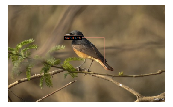
You can implement popular algorithms for object detection such as YOLO (You Only Look Once) with, e.g., the image.darknet package or the platypus package. Here is a tutorial using image.darknet. Here is an example code with platypus. Sigrid Keydana provides code to train a model from scratch on RStudio’s AI blog.

• Image classification: We have images of birds and we want the machine to tell us which bird is on a given image:

Sigrid Keydana has written a blog post on image classification using torch. Shirin Elsinghorst uses keras and tensorflow to classify fruits. On this blog you can find code to build an image recognition app, also with keras and tensorflow. And there are also a number of applied use cases in scientific publications on computer vision in R, such as this article in Nature which classifies algae with deep learning in R.

Image segmentation: The general strategy

So, luckily for us R users, there are more and more R resources for various tasks in computer vision! There is little, however, on the specific task of image segmentation. I’ve been searching for implementations of models such as Mask R-CNN in R and have not been lucky to date (see also this issue raised on RStudio’s github). You could of course build the architecture from scratch in keras, but this is typically not what you want when you want to quickly test some models for prototyping in an applied use case.

One of the image segmentation models that you can try out very quickly is the U-net model. For an introduction to this model, read Daniel Falbel’s and Sigrid Keydana’s post at RStudio’s AI blog. Apart from the unet package which they are using, this is also possible with Michał Maj’s platypus package. Since I couldn’t find example code for image segmentation and subsequent background removal, I decided to write this post hoping it might be of help to someone looking to do a similar project.

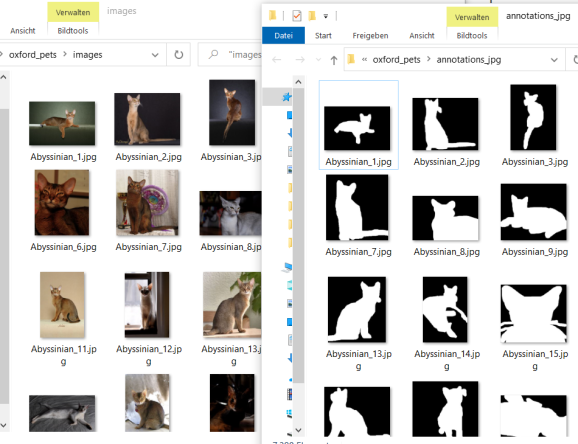
So what’s the plan? We first look for training data consisting of image pairs: For each image we need a mask delineating the foreground object later to be cropped. See the following screenshot as an example:

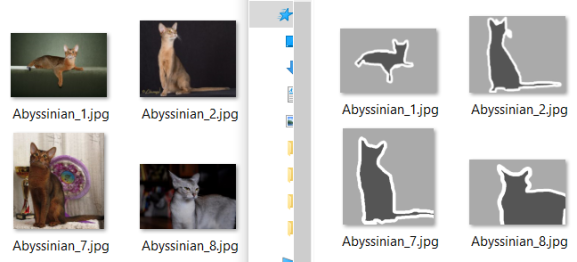
With these data, we train a deep learning model that classifies every pixel on the image as either “background” or “foreground” (or “border” in this case). Once we have trained a model that is capable of adequately classifying pixels into these categories on new, unseen images, we can apply the model to our own images.

Where do you get these training images from? In general, you can either

• load a pre-trained model from somewhere without any training done by yourself,
• generate your own training data, which means that you manually create masks of your images (so that you have two folders with images and corresponding masks as in the screenshot shown above), which would be ideal, because then you can train the model specifically to your use case, but generating masks can obviously be time-consuming, or
• train a model with training data found elsewhere and hope it performs reasonably well when applied to your data.

We are going to do the latter. We first load training images with corresponding masks of cats and dogs, train the model on these images, and then use the model for our own dataset of birds.

Loading and preparing the training data

We use the oxford pets dataset to train our model. Download the images and the annotations and extract them to two separate folders. In the “annotations” folder, we delete everything apart from the .png-files that match the names in the images folder.

So your two folders should look like this:

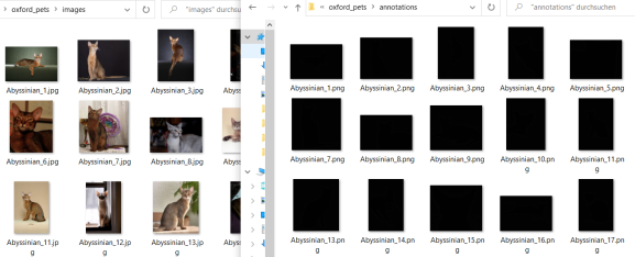
Note that I moved the annotation images from the “trimaps” folder into the superseding “annotations” folder and deleted all the other folders, for reasons of clarity. I also deleted all files starting with “_” as well as the “readme”, “list.txt”, “test.txt” and “trainval.txt” because we want to have matching images and masks and no other files in the two directories.

In the screenshot above you can see that the images are jpeg’s whereas the annotations are png’s. I converted all the png’s to jpg, which is of course not strictly necessary, but it makes things a bit easier, and also I want to apply some additional transformation to the images, so let’s write a small function to transform and convert all images:

library(tidyverse)
library(keras)
library(tensorflow)
#remotes::install_github("maju116/platypus")
library(platypus)
library(magick)
library(png)
library(jpeg)

setwd("C:/Users/my_name/Desktop/Image_Project")

dir.create("oxford_pets/annotations_jpg")

convert_batch <- function(x){
  mask1 <- readPNG(paste0("oxford_pets/annotations/",x))
  mask1 <- (mask1*255-1)/2
  mask1 <- ifelse(mask1<0.3 | mask1>0.7,1,0)
  writeJPEG(mask1, target = paste0("oxford_pets/annotations_jpg/",
                                   strsplit(x,".",fixed=T)[[1]][[1]],".jpg"), quality = 1)
}

sapply(dir("oxford_pets/annotations/"),convert_batch)

Let’s see what we did there: If you are missing any of these libraries, install them with install_packages() except for the platypus package which you can install from github with the command given in line 4. If this is your first time installing keras and tensorflow in R, you will have to run the following commands once each: install_keras(); install_tensorflow() after you installed them via install_packages().

After the libraries have been loaded, you obviously set your working directory to the path containing the two folders with the oxford pets and annotations in line 10 of the code chunk above. When you run the rest of the code, you get a new folder containing all the image masks as jpg’s:

In the code you can also see that we transformed the trimaps to have only values 0 or 1 for black and white. The reason for this is that the masks originally looked like this:

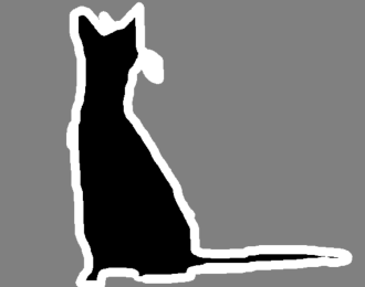
So they originally had three regions: foreground, background, and border. Which is great because you could later apply e.g. a small amount of blur onto the border pixels after you removed the background. But in order to keep things simple, in this tutorial we work with binary masks consisting only of foreground and background. If you do want to train a model that detects the three different types, just delete the line with the ifelse-statement in the code above.

You can then check whether there are any images in the “annotations_jpg” folder that are not contained in the “images” folder (and vice versa) as follows:

table(dir("oxford_pets/annotations_jpg/") %in% dir("oxford_pets/images/"))

table(dir("oxford_pets/images/") %in% dir("oxford_pets/annotations_jpg/"))

In my case there were three files in the image folder not matching the files in the annotations folder, which you can identify with:

dir("oxford_pets/images/")[which(!dir("oxford_pets/images/") %in% dir("oxford_pets/annotations_jpg/"))] 

Delete these three files and then you can also delete the old “annotations” folder with the png’s.

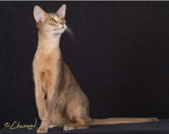
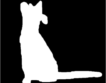
Show me some example image and corresponding mask in R:

image1 <- readJPEG("oxford_pets/images/Abyssinian_2.jpg")
plot(as.raster(image1))

mask1 <- readJPEG("oxford_pets/annotations_jpg/Abyssinian_2.jpg")
plot(as.raster(mask1))

Train the u-net model

Let’s initialize the u-net model with some standard parameters:

batch_size <- 32
size <- 256
n_training <- length(dir("oxford_pets/images/"))

test_unet <- u_net(size,size,
                    grayscale = F,
                    blocks = 4,
                    n_class = 2 #background + foreground
)

test_unet %>% compile(optimizer = optimizer_adam(lr=0.001),
                      loss = loss_dice(),
                      metrics = metric_dice_coeff())

test_unet

Which gives us the architecture of the u-net:

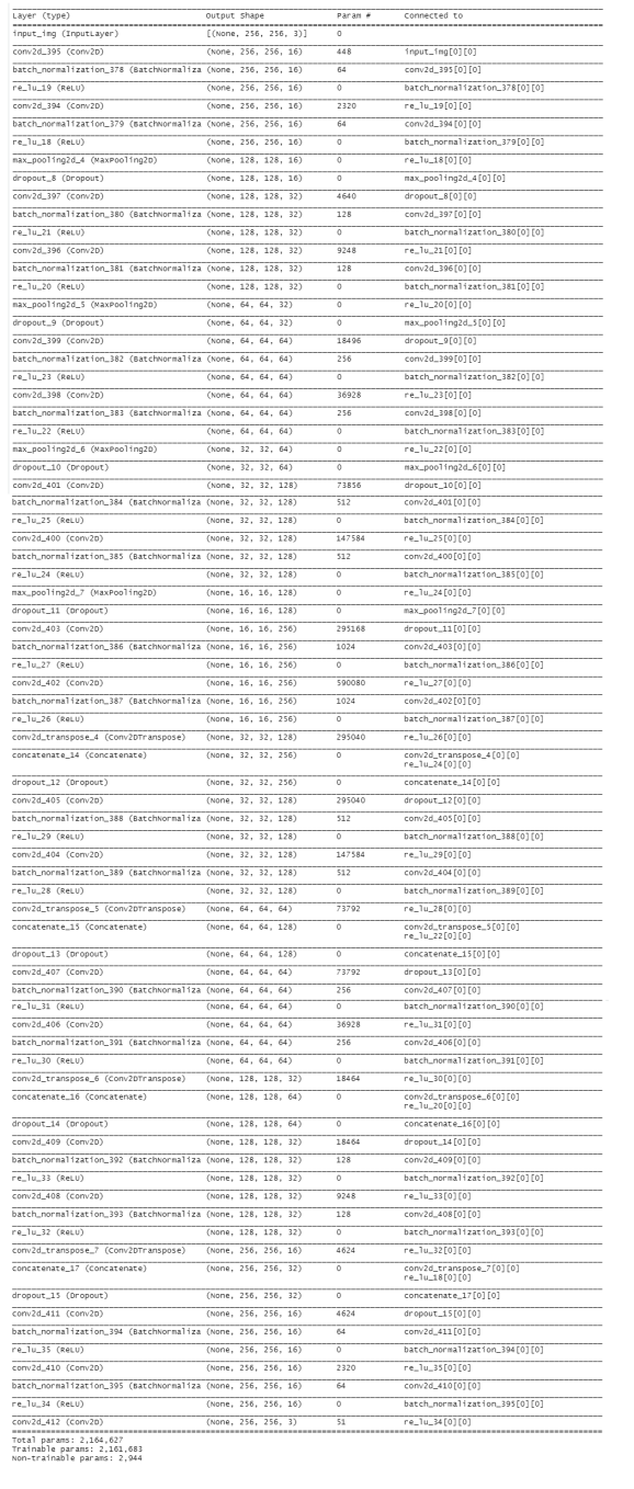
Thank you again to the people who took the time to port this into R, I wouldn’t want to build this from scratch not even with a tool as easy to use as keras. So here is hoping someone will be so kind as to do the same with the Mask R-CNN or the Faster R-CNN models…

In the meantime, let’s train our u-net model with the cats and dogs training data. We first define the data generator, specifying the locations of our images and masks, and setting some additional parameters:

datagen <- segmentation_generator(
  path = "oxford_pets",
  colormap = binary_colormap,
  only_images = F,
  mode = "dir",
  net_h = size, net_w = size,
  grayscale = F,
  batch_size = batch_size,
  shuffle = F,
  subdirs = c("/images", "/annotations_jpg")
)

Note that we set “colormap = binary_colormap” here because our masks consist only of black and white pixels. In case you want to classify background + foreground + border, you could define a new object like this:

trinity_colormap <- list(
  c(0,0,0), c(128,128,128), c(255,255,255)
)

and pass this object to the “colormap” argument of the segmentation_generator() function above. This works only if you also applied the converting function in the first code chunk above, because there we transformed the pixel values of all our masks to have exactly these values (0 = black, 255 = white, 128 = gray). If you’re unsure about the colors on your masks, read one in as with the readJPEG() function in the previous section and run table(mask1) to see which pixel values your masks have.

Now on to the actual training! I’m training the model for only 5 epochs here because I’m on my local laptop and this takes a while… If you need optimal results, you would of course set this to a higher value.

history <- test_unet %>%
  fit_generator(
    datagen,
    epochs = 5,
    steps_per_epoch = n_training %/% batch_size,
    verbose = 2
)

If you have used keras in RStudio before, then you are probably familiar with the following plot that is generated during training in our viewer pane:

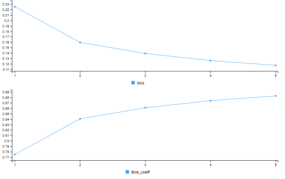
So after 5 epochs, our dice coefficient is at around 0.9, which is not bad. Remember that this statistic compares the predicted masks to the actual masks and calculates the harmonic mean of precision and recall just as the F1 score which is a common metric in machine learning. In simple words, in most of the cases where our model says “this pixel probably belongs to a foreground object”, the model is right. But there is of course still room for improvement. The easiest way to get better results here would of course be more training, and you could also optimize the learning rate. But let’s work with what we have achieved so far.

Once you are satisfied with the model’s (in-sample) performance, you can save the trained weights as follows:

save_model_weights_tf(test_unet, "unet_model_weights")

In a future session (or in a productive environment, say, on your server or in an app), after initializing the model as above, you just have to run load_model_weights_tf() and specify the path to your saved model weights.

Testing the model

We first use the model to draw masks from pictures. Having tested this, we write a function for automatic background removal.

Let’s first test the model with a cat image from our training data. This shouldn’t be a problem for the model since it was trained on these images:

cat <- image_load("oxford_pets/images/Egyptian_Mau_4.jpg", target_size = c(size,size))

cat %>%
  image_to_array() %>% 
  `/`(255) %>%
  as.raster() %>%
  plot()

Let the model generate a mask for this cat:

x <- cat %>% 
  image_to_array() %>%
  array_reshape(., c(1, dim(.))) %>%
  `/`(255)

mask <- test_unet %>% predict(x) %>%
  get_masks(binary_colormap)

plot(as.raster(mask[[1]]/255))

The result:

Compare to the ground truth, i.e. the mask provided with the training data for this image:

Well, not exactly the same, but better than nothing. Again, with more rounds of training we could boost the performance.

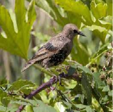
Now, let’s load a bird image – which the model has not been trained on – and tell the model to segment foreground from background:

bird <- image_load("birds_folder/starling female/020.jpg", target_size = c(size,size)) 

bird %>%
  image_to_array() %>% 
  `/`(255) %>%
  as.raster() %>%
  plot()

which gives us the original image:

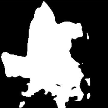
Now we feed this image to our trained model and get the predicted mask as output:

x <- bird %>% 
  image_to_array() %>%
  array_reshape(., c(1, dim(.))) %>%
  `/`(255)

mask <- test_unet %>% predict(x) %>%
  get_masks(binary_colormap)

plot(as.raster(mask[[1]]/255))

which gives us this results:

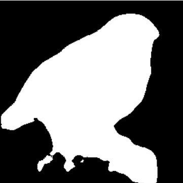
Doesn’t look so bad, although you can see that a part of the wooden post in the bottom right has been mistaken for a part of the bird.

Now I won’t lie, sometimes it doesn’t work quite as well:

Obviously – and you might know this from your Zoom/Teams/GMeet… concerences, when your fake background suddenly starts crumbling and your yucca palm or your wardrobe’s door become visible – when there’s a lot going on in the picture, the model might have greater difficulties discerning foreground object from background.

What could you do about this? Of course, if possible, try to get pictures with a smooth and uniform background. You could also try a more complex modelling pipeline. Think of, for instance, object detection + cropping around boundary boxes + subsequent image segmentation. And, of course, more training – and if possible, training on data relevant to the domain at hand. That is, train on bird images to get good results for birds, not on cats and dogs. But that’s beyond the scope of this post. Let’s look at what we can do with the model at hand.

Automatic background removal

We can now write a little function that reads an image, generates a mask with our trained model, uses the mask to remove the image’s background, and pastes the foreground object onto another background:

change_background <- function(image, background){
  img <- image_load(image, target_size = c(size,size))
  
  x <- img %>% 
    image_to_array() %>%
    array_reshape(., c(1, dim(.))) %>%
    `/`(255)
  
  mask <- test_unet %>% predict(x) %>%
    get_masks(binary_colormap) 
  
  mask_blur <- magick::image_read(mask[[1]]/255) %>%
    image_blur(20,5) 
  
  img_crop <- image_composite(image_read(image_to_array(img)/255), mask_blur,operator = "CopyOpacity")
                              
  background <- image_read(background)
  
  image_composite(background, img_crop, gravity = "center")
  
}

Quick summary of what this does: We load an image, transform it to the size that our Tensorflow model expects, predict the classes (foreground vs background) with our u-net model and extract the mask. Then I applied some amount of blur to the mask with magick’s image_blur() function. Next, the “img_crop” object is obtained by adding the mask onto the original image. Then we load a background image and paste our cropped foreground object onto the new background.

This is how you use the function:

change_background(image = "birds/owl/612.jpg",
                  background = "backgrounds/random_water.jpg")

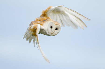
I’ve taken a picture of an owl which originally looked like this:

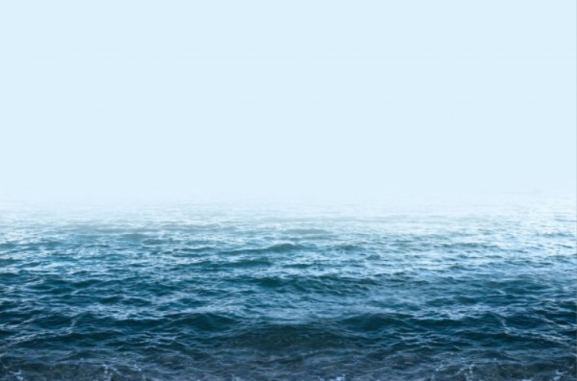
And a random picture of an ocean which originally looked like this:

Running our function gives you:

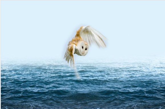
Aaalright, not quite publication-ready. Remember, you could improve these results by:

• longer model training,
• train three classes (background + foreground + border) as the original training images provided, and apply some special functions (blur, transparency…) to the border,
• domain-specific training data (here: images and masks of birds, not of dogs and cats),
• other algorithm (e.g. Mask R-CNN instead of U-Net),
• fine-tuning with magick inside the function (I bluntly applied some blur to the mask, you could think of more sophisticated operations here),
• etc.

But hopefully this code gives you some idea about where to start with a similar project.

One more try:

Original image:

Our function applied:

Alright, let’s leave it at that. As you can see, the results are not breathtakingly good. I’ve given some suggestions for improvements above – maybe some of you have other ideas, please let me know!

Thank you for your interest and good luck with your R projects!