Imagine you could:

1. Take a picture with your phone of a bird in your backyard.
2. Upload the foto to an app.
3. The app tells you what kind of bird it is.

In this tutorial, you will learn how to quickly build an app that does just that – using only the open-source software R.

In this first part, we’ll set up and train the machine-learning model. In a second post, I will give example code for an app that can be deployed online.

If you’re not interested in birds, think of other possible applications:

• Detection of defect parts/ scratches/… in an industrial production line,
• facial recognition,
• setting up a web-cam in my backyard and alert me if a specific type of animal runs through,
• etc.

Now you might say “there are already tons of apps for all these purposes”. Right, but when creating your own algorithm, you can tailor it for your specific application. For instance, your company might have specific quality issues with certain products and there is no out-of-the-box app that can discern them from good products. Or, as in our case here, I was interested in a model that identifies the >500 bird species that exist in the area where I live, but most of the datasets that I found online include predominantly North American birds.

Note that we won’t build a general-purpose app that can identify anything on an image. Rather, we build an image classification model, that is a supervised machine-learning algorithm which is trained on human-labelled images. In other words, you will provide the machine with training data – say, 40 folders with many images of 40 different bird species. Or two folders labelled “defect machines” and “ok machines”, if your use case were a binary defects-detection classification.

This means of course that the app can only identify the bird species that you trained it on. But it will be able to classify previously unseen images without you needing to tell the system what to look for. This is the reason why machine-learning has revolutionized computer vision: There is no need to hard-code rules (such as “if it has black feathers and an orange bill, then it might be a blackbird, except if…”), the system learns quasi-autonomously.

Up until a few years ago, image classification was a difficult task that only highly-trained experts with access to expensive computing systems were able to accomplish. Then came the so-called “ImageNet moment” in 2012, when researchers used new kinds of neural networks to achieve dramatically better results than anyone ever before in the ImageNet competition that involves classifying millions of images into 20,000 categories. As of 2021, the best-performing algorithms achieve around 90% accuracy in this task whereas by 2011, the best result was only 50%. This shows the incredible progress this field has made in only a few years. Unsurprisingly, deep learning has received huge attention in academia and beyond, with the top cited articles in Nature in the last years predominantly belonging to the field of artificial neural networks. It’s worth reading this overview article in Nature written by three of the most prominent authors in the field.

In the last few years, frameworks such as keras have allowed these algorithms to be implemented by basically anyone with a laptop and an internet access. The relevant libraries for large-scale tensor manipulation for deep learning such as Tensorflow or PyTorch are all written for Python. Hence, by far the majority of people use Python for deep learning. The hype around neural networks is the major reason for why Python has overtaken R as the most popular programming language for data science.

If you’re an R user (like me), you might be wondering if you can implement neural networks with Keras and Tensorflow in R as well – you can! Of course you could switch to Python for your deep learning models. The reason why one might want to do it in R is that as an R user, you are probably much more comfortable and efficient processing your data with the tidyverse or data.table, visualizing it with ggplot2 or publishing it with shiny or RMarkdown. So in order to avoid system discontinuities you can do your entire project in R and call the relevant Python libraries from within R.¹

For an in-depth understanding of deep learning in R, read Francois Chollet’s (developer of Keras) and J.J. Allaire’s (RStudio founder) book. For a quick overview, continue reading this post.

Getting started

Start RStudio and load the following packages (install if necessary):

library(tidyverse)
library(keras)
library(tensorflow)
library(reticulate)

If this is your first time running keras and tensorflow, you will need to enter

install_tensorflow(extra_packages="pillow")
install_keras()

into the console once. Pillow (PIL) is a Python package that is needed for image processing later. During the installation process, you will be asked if you want to install Python through miniconda if you have no Python distribution on your computer. (If not, install e.g. Anaconda (or Miniconda) manually).

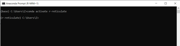
If you run into troubles at this or a later point regarding Pillow/PIL, you can try the following: Start Anaconda’s command prompt (on Windows, hit the start button and type “Anaconda” to search for the prompt). Enter “conda activate r-reticulate” to activate the virtual environment for Python use in R and then enter “conda install pillow”. As yet another alternative, enter “reticulate::py_install(“pillow”)” into the R console. Hopefully one of those steps gets you going…

Load training data

For demonstration purposes, we will download an existing dataset of birds and train the algorithm on it. [What I did for my actual app, by contrast, and what you will probably need to do if you have a specific use case, is assemble your own training data. For instance, you take fotographs of a few hundred defect/ok machines and save them into folders named “defect” and “ok”, respectively. In my case, I assembled data from the internet on specific birds species that are common in my area but aren’t included in the large datasets that can be found online. Obviously, generating training data is often the most time-consuming part in a data science project.]

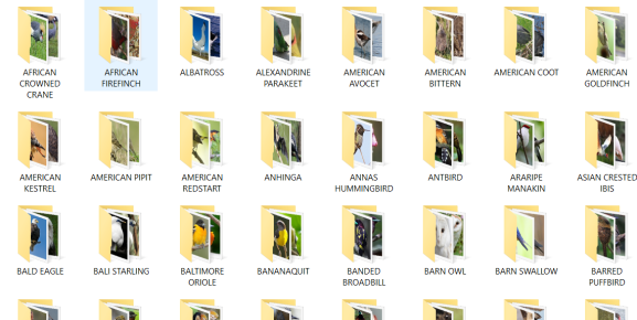
Download the 250 birds species dataset from Kaggle. For reasons of computing performance, I limit the data to the first 40 birds in this example (from “African Crowned Kane” to “Blue Heron”). So you should have folders “train” and “test” with 40 subfolders each with images for training and testing for each of the 40 bird species. (There is also a validation folder but we will create the training/validation split in the code to make it more generalizable).

In R, set your working directory to the folder where all the images are located. With the dir() command, we get a list of all birds in the correct order and save it for later purposes:

setwd("C:/users/my_name/desktop/birds")
label_list <- dir("train/")
output_n <- length(label_list)
save(label_list, file="label_list.R")

Now we set the target size to which all images will be rescaled (in pixels):

width <- 224
height<- 224
target_size <- c(width, height)
rgb <- 3 #color channels

After we set the path to the training data, we use the image_data_generator() function to define the preprocessing of the data. We could, for instance, pass further arguments for data augmentation (apply small amounts of random blurs or rotations to the images to add variation to the data and prevent overfitting) to this function, but let’s just rescale the pixel values to values between 0 and 1 and tell the function to reserve 20% of the data for a validation dataset:

path_train <- "/train/"
train_data_gen <- image_data_generator(rescale = 1/255, 
  validation_split = .2)

The flow_images_from_directory() function batch-processes the images with the above defined generator function. With the following call you assign the folder names in your “train” folder as class labels, which is why you need to make sure that the sub-folders are named according to the bird species as shown in the second picture above. We create two objects for the training and validation data, respectively:

train_images <- flow_images_from_directory(path_train,
  train_data_gen,
  subset = 'training',
  target_size = target_size,
  class_mode = "categorical",
  shuffle=F,
  classes = label_list,
  seed = 2021)

which gives us the confirmation about how many images were loaded:

validation_images <- flow_images_from_directory(path_train,
 train_data_gen, 
  subset = 'validation',
  target_size = target_size,
  class_mode = "categorical",
  classes = label_list,
  seed = 2021)

Note again that we do not use separate folders for training and validation in this example but rather let keras reserve a validation dataset via a random split. Otherwise we would have passed a different file path to the “validation_images” object and removed the “subset” arguments (and the “validation_split” argument in the image_data_generator() function above).

Let’s see if it worked:

table(train_images$classes)

This corresponds to the number of pictures in each of our folder, so everything looks good so far.

Show us an example image:

plot(as.raster(train_images[[1]][[1]][17,,,]))

The first element of our train_images object has the pixel values of each image which is a 4D-tensor (number of image, width, height, rgb channel), so with this call we are plotting image number 17.

Train the model

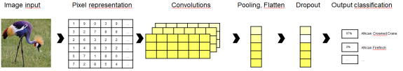
We are going to train a convoluted neural network (CNN). Intuitively, a CNN starts by sliding a smaller window across the input image and calculating the convolution of neighboring pixel values. This is like the cross-correlation of nearby values such that neighboring pixels with similar colors vs. sharp contrasts cause the convolution to take on different values. That way, prominent features such as edges can be detected regardless of their position in the image. This makes CNNs much better at image recognition as opposed to standard neural networks that would take e.g. a 224×224 feature vector as an input and disregard whether key aspects of the image (e.g. the bird’s head) appear on the top left or rather the bottom right of the picture.

Now, the great flexibility of neural networks that enables them to learn any kind of function comes at a cost: There are millions of different ways to set up such a model, and depending on the values of parameters that most people have no idea what they are doing, your model might end up with anything between 3% and 99% accuracy for the task at hand. [This is the well-known bias-variance tradeoff: A linear regression is very well understood and there is nothing you can “tune” about it given a set of predictor variables, so 10 different researchers will ususally obtain 10 identical results (i.e. the model’s variance is low). But the model assumptions (linear relations between all predictors and the outcome, no collinearity between the predictors, and so on) are typically violated, so the model is biased. By contrast, a neural network can learn non-linear relations, interaction effects, etc., but has a huge variability depending on various “hyperparameters” such as the number of neurons in a hidden layer, the learning rate of the optimizer, etc.]

Luckily, there is a way to quickly generate good baseline results: Loading pre-trained models that have proven well in large-scale competitions such as the above-mentioned ImageNet. Here, we load the xception-network with the weights pre-trained on the ImageNet dataset – except for the final layer (which classifies the images in the ImageNet dataset) which we’ll train on our own dataset. We achieve that by setting “include_top” to FALSE in the following call:

mod_base <- application_xception(weights = 'imagenet', 
   include_top = FALSE, input_shape = c(width, height, 3))
freeze_weights(mod_base) 

Now let’s write a small function that builds a layer on top of the pre-trained network and sets a few parameters to variabes that we can later use to tune the model:

model_function <- function(learning_rate = 0.001, 
  dropoutrate=0.2, n_dense=1024){
  
  k_clear_session()
  
  model <- keras_model_sequential() %>%
    mod_base %>% 
    layer_global_average_pooling_2d() %>% 
    layer_dense(units = n_dense) %>%
    layer_activation("relu") %>%
    layer_dropout(dropoutrate) %>%
    layer_dense(units=output_n, activation="softmax")
  
  model %>% compile(
    loss = "categorical_crossentropy",
    optimizer = optimizer_adam(lr = learning_rate),
    metrics = "accuracy"
  )
  
  return(model)
  
}

We let this model compile once with our base values and inspect its architecture:

model <- model_function()
model

which gives us:

Here we see that we have set the 20 Million parameters from the xception model to non-trainable, i.e. we only train our top layer, which is in this case a 1024×1 feature vector densely connected to the output classification layer. You can think of this feature vector as 1024 variables, each taking on specific values if a bird’s image has certain properties – say, if a bird has an orange tail then node 34 of this layer takes a high value. This is learned during the convolution layers of the xception network. There are ways of opening up this “black box” of how and why the network arrives at its predictions (see, for instance, the lime package), which is good if you want to fine-tune the architecture, but let’s start with training the model as is:

batch_size <- 32
epochs <- 6

hist <- model %>% fit_generator(
  train_images,
  steps_per_epoch = train_images$n %/% batch_size, 
  epochs = epochs, 
  validation_data = validation_images,
  validation_steps = validation_images$n %/% batch_size,
  verbose = 2
)

Depending on your hardware (local laptop vs. cluster, parallel computing, GPU’s/TPU’s etc.) this may take a few minutes up to an hour. In RStudio, we get a nice graph showing how in-sample and out-of sample (validation) loss and accuracy evolved with each step of adjusting the weights of our network. Note that if you suspect that validation accuracy would have increased beyond the 6 steps, set “epochs” to a higher value. If your model is already over-fitting, i.e. validation value accuracy decreaes while training accuracy further increases, you could even cut down on the number of epochs. In our case here, we achieve around 89% accuracy in the validation dataset after 6 epochs. Not a bad start but it can certainly be improved, which we will look into later.

Evaluating and testing the model

Let’s see how well our model classifies the birds in the hold-out test dataset. We use the same logic as above, creating an object with all the test images scaled to 224×224 pixels as set in the beginning. Then we evaluate our model on these test images:

path_test <- "/test/"

test_data_gen <- image_data_generator(rescale = 1/255)

test_images <- flow_images_from_directory(path_test,
   test_data_gen,
   target_size = target_size,
   class_mode = "categorical",
   classes = label_list,
   shuffle = F,
   seed = 2021)

model %>% evaluate_generator(test_images, 
                     steps = test_images$n)

The result:

Not a bad start!

We can also upload a custom image to see what our model predicts. Here I took an image of a bald eagle (making sure it’s not one of the training images) and fed it to the model:

test_image <- image_load("Test images/Bald Eagle/index.jpg",
                                  target_size = target_size)

x <- image_to_array(test_image)
x <- array_reshape(x, c(1, dim(x)))
x <- x/255
pred <- model %>% predict(x)
pred <- data.frame("Bird" = label_list, "Probability" = t(pred))
pred <- pred[order(pred$Probability, decreasing=T),][1:5,]
pred$Probability <- paste(format(100*pred$Probability,2),"%")
pred

This gives a nice overview of the model’s predictions:

Okay, that wasn’t so hard. But let’s see if the model has more problems with the Baltimore Oriole or the Bananaquit…

To further investigate this, let’s look at exactly which birds are well vs. not so well identified by our model. Shirin Elsinghorst made a great post about that. I have a slightly different approach here but the outcome is similar. We first generate a matrix of all predictions for each image in the test dataset (= rows) to all bird species (columns). Then we label the highest prediction for each image as “predicted_class” and compare it with the actual class. Finally, we count the percentage of correct classifications (since each of our class has exactly 5 test images, the values will be either 0, 20, 40, 60, 80 or 100%) and plot the results:

predictions <- model %>% 
  predict_generator(
    generator = test_generator,
    steps = test_generator$n
  ) %>% as.data.frame

names(predictions) <- paste0("Class",0:39)

predictions$predicted_class <- 
  paste0("Class",apply(predictions,1,which.max)-1)
predictions$true_class <- paste0("Class",test_generator$classes)

predictions %>% group_by(true_class) %>% 
  summarise(percentage_true = 100*sum(predicted_class == 
    true_class)/n()) %>% 
    left_join(data.frame(bird= names(test_generator$class_indices), 
    true_class=paste0("Class",0:39)),by="true_class") %>%
  select(bird, percentage_true) %>% 
  mutate(bird = fct_reorder(bird,percentage_true)) %>%
  ggplot(aes(x=bird,y=percentage_true,fill=percentage_true, 
    label=percentage_true)) +
  geom_col() + theme_minimal() + coord_flip() +
  geom_text(nudge_y = 3) + 
  ggtitle("Percentage correct classifications by bird species")

[Note that in Python row and column indices start with 0 whereas in R they start with 1, which is why I’m pasting class names 0:39 to match the keras class names, but when getting indices from R functions (which.max()) I have to substract 1 because they return 1:40.]

This gives the following output:

Great – now we know which bird species our model has problems with so far. The Baltimore Oriole didn’t prove to be a problem but the Bananaquit apparently did.

Tuning the model

So what can we do about that? We could either assemble more (and different) training data for the birds we currently have problems identifying. And/or we could tune our model, since we went with the first configuration that came to mind so far.

There are various approaches to model tuning. We will present a very crude one here which, in keeping with the blog’s name, involves a nested for-loop. We first define a grid with values for our parameters that we seek to optimize. Then we loop over each combination of parameters, fit the model and save the model combination and final validation accuracy:

tune_grid <- data.frame("learning_rate" = c(0.001,0.0001),
                        "dropoutrate" = c(0.3,0.2),
                        "n_dense" = c(1024,256))

tuning_results <- NULL
set.seed(2021)

for (i in 1:length(tune_grid$learning_rate)){
  for (j in 1:length(tune_grid$dropoutrate)){
      for (k in 1:length(tune_grid$n_dense)){
        
        model <- model_function(
          learning_rate = tune_grid$learning_rate[i],
          dropoutrate = tune_grid$dropoutrate[j],
          n_dense = tune_grid$n_dense[k])
        
        hist <- model %>% fit_generator(
          train_images,
          steps_per_epoch = train_images$n %/% batch_size, 
          epochs = epochs, 
          validation_data = validation_images,
          validation_steps = validation_images$n %/% 
            batch_size,
          verbose = 2
        )
        
        #Save model configurations
        tuning_results <- rbind(
          tuning_results,
          c("learning_rate" = tune_grid$learning_rate[i],
            "dropoutrate" = tune_grid$dropoutrate[j],
            "n_dense" = tune_grid$n_dense[k],
            "val_accuracy" = hist$metrics$val_accuracy))
        
    }
  }
}

tuning_results

This gives you an overview of all the used hyperparameter combinations and the outcome. Select the best performing model with, e.g.:

best_results <- tuning_results[which( 
  tuning_results[,ncol(tuning_results)] == 
  max(tuning_results[,ncol(tuning_results)])),]

Now you have a general idea whether you should change your tune_grid to much higher or lower values of the learning rate, dropout rate, etc. The downside to this approach here is (apart from the obvious crudeness vis-à-vis more sophisticated approaches such as LR finder) that once you have identified the best performing model, you need to train it once again and then save it for further use:

model <- model_function(learning_rate = 
  best_results["learning_rate"],
  dropoutrate = best_results["dropoutrate"],
  n_dense = best_results["n_dense"])

hist <- model %>% fit_generator(
  train_images,
  steps_per_epoch = train_samples %/% batch_size, 
  epochs = epochs, 
  validation_data = validation_images,
  validation_steps = valid_samples %/% batch_size,
  verbose = 2
)
model %>% save_model_tf("bird_mod")

Next time you want to use the model (e.g. in your app), load it with load_model_tf().

Summary

With minimal effort, we trained and evaluated an algorithm that is able to classify previously unseen images of birds into 40 species with a 92% accuracy. With some additional efforts – training data collection, data augmentation, hyperparameter tuning… – we could surely further improve this performance. Once you’re more advanced in this topic, you could think of tailoring the network architecture to your use case, use additional nets for feature engineering (say, you have one model only looking for bird eye color and save the result as a feature to your final model; or you could start with a model detecting bird vs. background, crop the bird and paste it onto a blank background, and then feed it to the subsequent model), and so on.

In the next post, I will use this model and deploy it as a shiny app which can be used on your computer or phone. Thank you for your interest and good luck with your projects!

—

¹Please don’t mistake this for a Python vs. R discussion. There are countless reasons to use Python for various tasks and I am in fact using it too to, e.g., put machine learning models into production. But when you come from a discipline more engaged with “classical” (explanatory) statistics, you are probably trained in R because as fas as I know, it would be much more difficult running a, say, repeated-measures ANOVA or a fixed-effects panel regression in Python. Of course there are certainly libraries for that nowadays, but the methodological advances in fields such as Economics, Medicine, or Psychology are most often implemented in R with a citable publication in a statistical journal, so in many academic fields R is still the de-facto standard. So if you’re like me a result of the over-production of academics in some of these fields, you might need to broaden your horizon and get involved with the predictive modeling paradigm but still want to use R as your primary language for quick prototyping and data manipulation, and that is what this blog post is for.