Venn diagrams are a great way to visualize informative comparisons between data sets. It can be particularly helpful to use venn diagrams to look at how similar data is across multiple data sets, or within the same data set.

The types of comparisons you can make will depend on how your data is formatted. In the following example we will use the counts of differentially expressed (DE) genes to compare the following six different Daphnia genotypes.

Genotype	Species	Region
PA	Daphnia pulex	Portland Arch, IN
Y023	Daphnia melanica	Olympic Mountains, WA
R2	Daphnia melanica	Olympic Mountains, WA
Y05	Daphnia melanica	Olympic Mountains, WA
E05	Daphnia melanica	Olympic Mountains, WA
Sierra	Daphnia melanica	Sierra Nevada, CA

Venn Diagram Script – R

The following R scripts will be used to generate several different venn diagrams for a variety of comparisons across genomic data sets.

The first step is to import a package for creating venn diagrams in R. Here we will use the VennDiagram library.

#install.packages('VennDiagram')
library(VennDiagram)

---

Next, the read.csv function is used to import the genomic data we want to analyze. The path to the data being imported is set as an input to the script using args[1].

The format of the data is expected to be a table of gene counts where the rows are counts by gene ID, and columns are counts by genotype.

#Import data
counts <- read.csv(file=args[1])

---

Now that the data we are going to analyze is imported to the counts data frame, we can subset the data to make informative comparisons.

Remember that in this example, the imported data are the counts of differentially expressed (DE) genes for six different genotypes. So the following subsets of SET1 to SET6 represent the counts for each of the six genotypes.

Also note that the subset of data for each genotype is taken from a column of the same name in the imported csv data (Y05, Y023, E05, R2, PA, and Sierra). This means that the column name tags will need to be changed to the columns of your input data set that you wish to use for comparisons.

#Define sets for diagram
SET1 <- counts$Y05
SET2 <- counts$Y023
SET3 <- counts$E05
SET4 <- counts$R2
SET5 <- counts$PA
SET6 <- counts$Sierra

---

Before the venn diagrams can be generated all NA values need to be replaced with empty strings using the is.na function. This is because any NA in the data set will cause an error when creating the diagrams.

Although, you should be sure that the presence of NA values in your data set is not a cause for concern. It is not uncommon for NAs to be found in counts of gene expression data produced by some quantification programs.

#Replace NAs
SET1[is.na(SET1)] <- ""
SET2[is.na(SET2)] <- ""
SET3[is.na(SET3)] <- ""
SET4[is.na(SET4)] <- ""
SET5[is.na(SET5)] <- ""
SET6[is.na(SET6)] <- ""

---

Now we are ready to begin generating venn diagrams in R. There are a number of comparisons we can make since we are working with six data sets in this example, one for each genotype.

The first comparison we will make is of the counts of DE genes between the four D. melanica genotypes (Y05, E05, Y025, R2) from the same geographic region and the D. pulex out group (PA).

Note that the venn.diagram function from the VennDiagram library has a variety of style options. Here we will use the fill option to set the colors for our data sets, and alpha to set the transparency. We can also save the diagram images to memory using the jpeg R function.

#Draw the diagram comparing the Olympics and PA sets
v2 <- venn.diagram(list(Y05=SET1, E05=SET3, Y023=SET2, R2=SET4, PA=SET5),
                   fill = c("red", "green", "white", "blue", "yellow"),
                   alpha = c(0.5, 0.5, 0.5, 0.5, 0.5),
                   filename=NULL)
jpeg("plotOlympicsPAVennn.jpg")
grid.newpage()
grid.draw(v2)
dev.off()

---

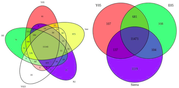
Next, we will compare the counts of DE genes across the four Olympics D. melanica genotypes and the closely related D. melanica from the Sierra Nevadas in CA (Sierra).

#Draw the diagram comparing the Olympics and Sierra sets
v3 <- venn.diagram(list(Y05=SET1, E05=SET3, Y023=SET2, R2=SET4, Sierra=SET6),
                   fill = c("red", "green", "white", "blue", "yellow"),
                   alpha = c(0.5, 0.5, 0.5, 0.5, 0.5),
                   filename=NULL)
jpeg("plotOlympicsSierraVennn.jpg")
grid.newpage()
grid.draw(v3)
dev.off()

---

Since this is differential gene expression data, we are also interested in comparing DE gene counts across the three genotypes that are tolerant to the treatment in our study.

#Draw the diagram comparing the tolerant sets
v4 <- venn.diagram(list(Y05=SET1, E05=SET3, Sierra=SET6),
                   fill = c("red", "green","blue"),
                   alpha = c(0.5, 0.5, 0.5), cat.cex = 1.5, cex=1.5,
                   filename=NULL)
jpeg("plotTolerantVenn.jpg")
grid.newpage()
grid.draw(v4)
dev.off()

---

Finally, we are interested in comparing DE gene counts across the three genotypes that are not tolerant to the treatment in our study.

#Draw the diagram comparing the non-tolerant sets
v5 <- venn.diagram(list(Y023=SET2, R2=SET4, PA=SET5),
                   fill = c("red", "green","blue"),
                   alpha = c(0.5, 0.5, 0.5), cat.cex = 1.5, cex=1.5,
                   filename=NULL)
jpeg("plotNonTolerantVennn.jpg")
grid.newpage()
grid.draw(v5)
dev.off()

---