
Package lconnect: patch connectivity metrics and patch prioritization
Want to share your content on R-bloggers? click here if you have a blog, or here if you don't.
Today I’m revisiting an older blog post on our package lconnect, which is available in CRAN (here). If you want to learn about the available connectivity metrics check this post.
It is intended to be a very simple approach to derive landscape connectivity metrics. Many of these metrics come from the interpretation of landscape as graphs.
Additionally, it also provides a function to prioritize landscape patches based on their contribution to the overall landscape connectivity. For now this function works only with the Integral Index of connectivity, by Pascual-Hortal & Saura (2006).
Here’s a brief tutorial!
First install the package:
#load package from CRAN
#install.packages("lconnect")
library(devtools)
Then, upload the landscape shapefile …
#Load data
vec_path <- system.file("extdata/vec_projected.shp", package = "lconnect")
…and create a ‘lconnect’ class object:
#upload landscape
land <- upload_land(vec_path, habitat = 1, max_dist = 500)
class(land)
## [1] "lconnect"
And now, let’s plot it:
plot(land, main="Landscape clusters")

If we wish we can derive patch importance (the contribution of each individual patch to the overall connectivity):
land1 <- patch_imp(land, metric="IIC")
##  [1]  0.0000000  0.0000000  0.0000000  0.0000000  0.0000000  0.1039501
##  [7]  0.1039501  0.0000000  0.1039501  0.0000000  0.0000000  0.1039501
## [13]  0.3118503 21.9334719  0.0000000 15.5925156  2.5987526  0.1039501
## [19]  0.1039501  0.2079002  0.0000000  0.0000000  0.0000000  0.0000000
## [25]  0.9355509  0.0000000 14.2411642  2.9106029  0.2079002 12.9937630
## [31]  0.3118503  0.7276507  0.0000000  7.5883576  0.5197505 70.2702703
class(land1)
Which produces an object of the class ‘pimp’:
## [1] "pimp"
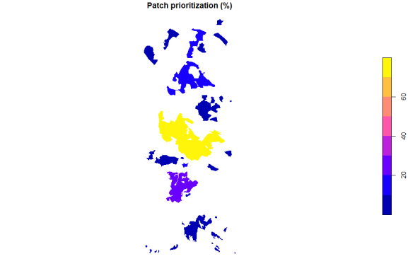
And, finally, we can also plot the relative contribution of each patch to the landscape connectivity:
plot(land1, main="Patch prioritization (%)")
And that’s it!
R-bloggers.com offers daily e-mail updates about R news and tutorials about learning R and many other topics. Click here if you're looking to post or find an R/data-science job.
Want to share your content on R-bloggers? click here if you have a blog, or here if you don't.