[This article was first published on Weird Data Science, and kindly contributed to R-bloggers]. (You can report issue about the content on this page here)
Want to share your content on R-bloggers? click here if you have a blog, or here if you don't.
To address this question we will delve once more into the arcana of machine learning, and draw out the technique of changepoint analysis. This procedure aims to identify one or more points in a series of observations at which the underlying process that generates the data has somehow altered.
Once more, we will operate within the warm embrace of Bayesian statistics and exploit the Stan modelling language as our means to cast light into the darkness2.
Reproducing, with only slight adaptations, the original Poisson example, our full joint probability would be:
The result is that our Stan model can be constructed by sampling across values of \(\theta_e\) and \(\theta_l\) for all possible values of \(c\). Due to the requirement to sum across all possible values of the discrete paramete, however, this subterfuge of marginalisation is restricted in general to bounded discrete parameters.
We can distill the above into a Stan model as given below.
Multinomial changepoint model
multinomial_changepoint.stan
data {

	int<lower=0> num_obs;				// Number of observations (rows/pages) in data.
	int<lower=0> num_cats;				// Number of categories in data.
	int y[num_obs, num_cats];  			// Matrix of observations.

	vector<lower=0>[num_cats] alpha;		// Dirichlet prior values.

}

transformed data {

	// Uniform prior across all time points for changepoint.
	real log_unif;
	log_unif = -log(num_obs);

}

parameters {

	// Two sets of parameters.
	// One (early) before changepoint, one (late) for after.
	simplex[num_cats] theta_e;
	simplex[num_cats] theta_l;

}

transformed parameters {

	//	// This code shows a slower, but easier to understand updating of log posterior via summation.
	//  vector[num_obs] lp;
	//  lp = rep_vector(log_unif, num_obs);
	//  for (s in 1:num_obs)
	//    for (t in 1:num_obs)
	//      lp[s] = lp[s] + multinomial_lpmf(y[t,] | t < s ? theta_e : theta_l);

	// This approach relies on dynamic programming to reduce runtime from quadratic to linear in num_obs.
	// See <https://mc-stan.org/docs/2_19/stan-users-guide/change-point-section.html>
		vector[num_obs] log_p;
	{
		vector[num_obs + 1] log_p_e;
		vector[num_obs + 1] log_p_l;

		log_p_e[1] = 0;
		log_p_l[1] = 0;

		for( i in 1:num_obs ) {
			log_p_e[i + 1] = log_p_e[i] + multinomial_lpmf(y[i,] | theta_e );
			log_p_l[i + 1] = log_p_l[i] + multinomial_lpmf(y[i,] | theta_l );
		}

		log_p =
			rep_vector( -log(num_obs) + log_p_l[num_obs + 1], num_obs) +
			head(log_p_e, num_obs) - head(log_p_l, num_obs);
	}
}

model {

	// Priors
	theta_e ~ dirichlet( alpha );
	theta_l ~ dirichlet( alpha );

	target += log_sum_exp( log_p );

}

generated quantities {

	simplex[num_obs] changepoint_simplex;	// Simplex of locations for changepoint.

	// Convert the log posterior to a simplex.
	changepoint_simplex = softmax( log_p );

}
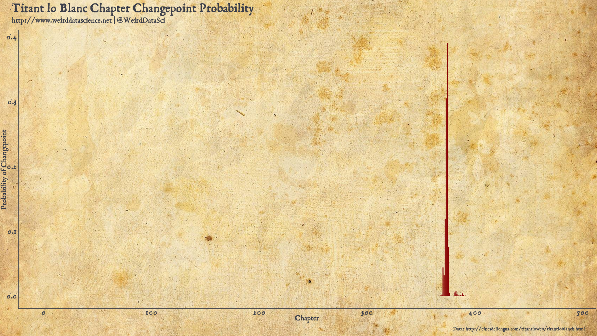
To launch the model in gentler waters, we apply it to Martorel and de Galba’s Tirant lo Blanc to discover where, if at all, de Galba’s major contributions to the text begin, and see the extent to which our Stan rendering reproduces the results of Riba and Ginebra’s analysis. As in their work we will focus only on those words with length shorter than 5 letters, where the key stylistic difference between authors makes itself apparent.
We place a relative uninformative Dirichlet prior on the multinomial \(\theta_e\) and \(\theta_l\) parameters, with the vector of \(\alpha\) values set to one. This results in a uniform distribution across all possible simplexes. Note that this does not push the multinomial towards a uniform simplex, but instead that all possible simplexes are equally likely. \(\alpha \ge 1\) produces increasingly uniform simplexes; \(0 \le \alpha \le 1\) produces simplexes in which the probability mass is more likely to be concentrated in some given element.
With the resulting data and model in unison, we can see the results of this analytic process.
Our multinomial automaton suggests a location for a significant stylistic changepoint in Tirant lo Blanc with the main concentration of probability mass around chapter 374. Perhaps unsurprisingly, but pleasingly, this is in close agreement with the earlier analysis of Riba and Ginebra, who placed their estimates between chapters 371 and 382.
The changepoint model realises the dark imaginings of our predecessors. What horrors might it reveal when applied to the Voynich Manuscript? Following the logic of the above analysis, we will focus initially on the shorter words in the Voynich corpus.
To improve model fit we will place a little more information in the prior, setting the \(\alpha\) values for the Dirichlet prior to 0.6 to push the multinomial towards more concentrated probabilities. This reflects the gamma distribution of word length frequencies discussed in our earlier analysis. We also combine all single- and two-letter Voynich terms into a single category due to the small number of words falling into these categories3.
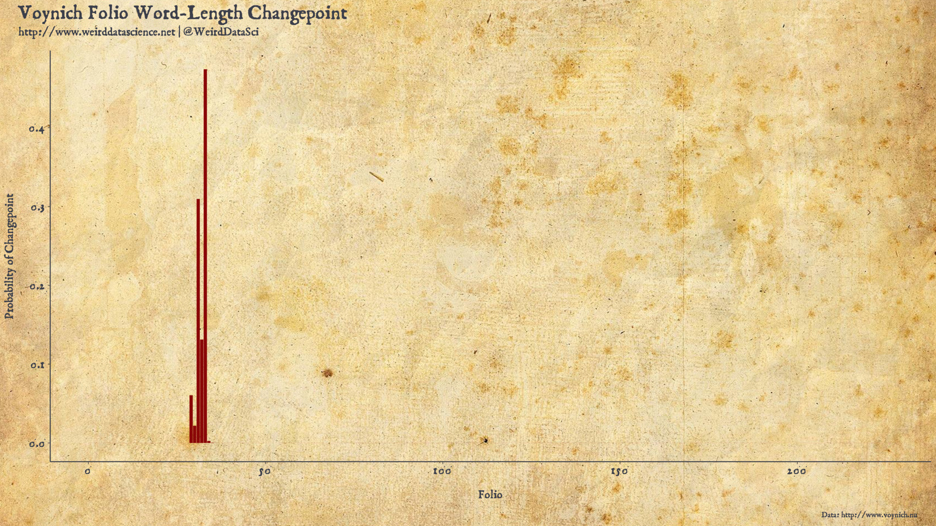
The model can now reveal where, if at all, a likely fracture resides in the textual assemblage of the Voynich Manuscript.
Our model appears to identify a potential changepoint in the frequency of short words in the Voynich Manuscript somewhere around Folio 33.
In contrast to the analysis of Tirant lo Blanc, we have no a priori suspicion that multiple authors were involved in the creation of the Voynich Manuscript. As such, we may hypothesise this changepoint as reflecting a simple stylistic shift, a shift in content, or, as with the previous analysis, a shift in authorship.
Mutatis Mutandis
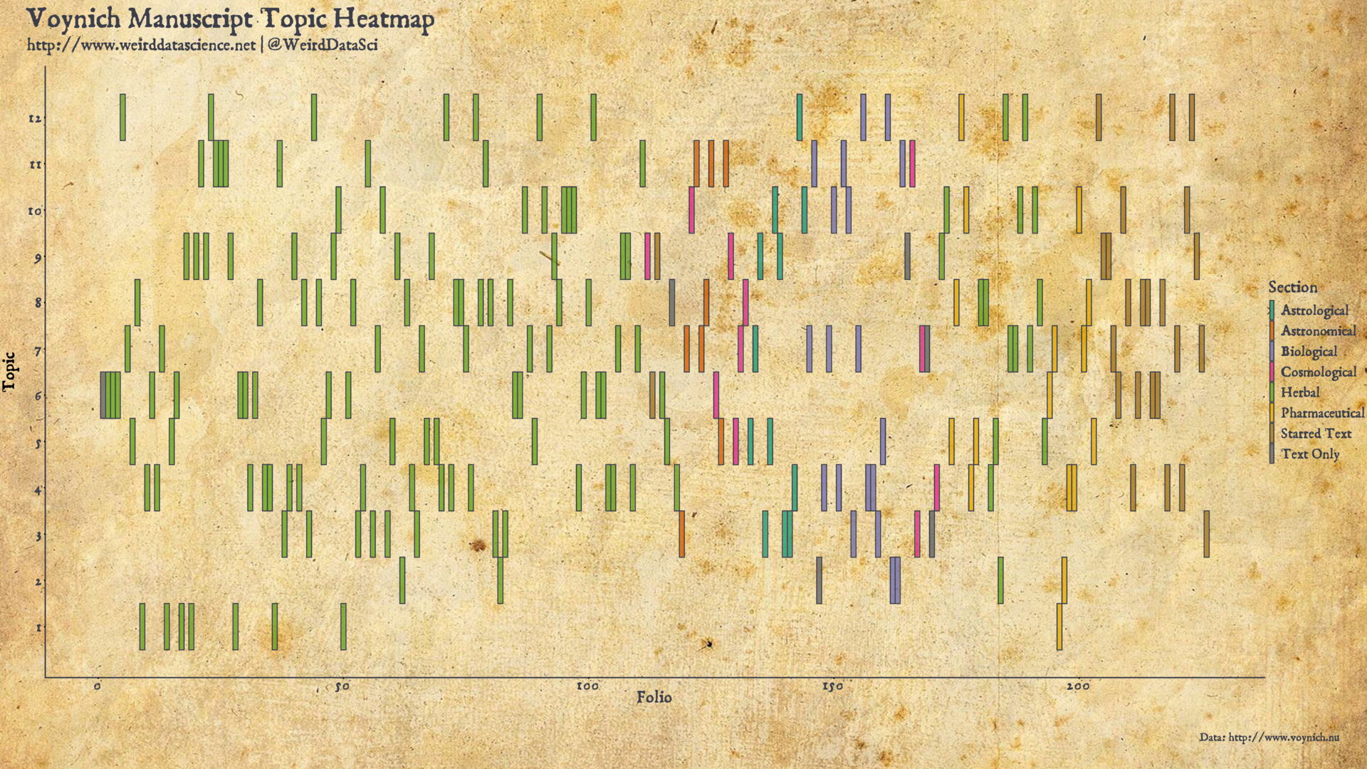
Recalling the topic model from the previous post, and the manually-assigned topics hinted at by the diagrams in the manuscript, Folio 33 might not immediately arouse our suspicions as the most obvious candidate for such a shift in style, falling as it does some way through the manually-identified herbal section, and without an immediately apparent shift in the distribution of topics.
For simplicity of presentation and analysis we will work with the alternative 12-topic model suggested by the metrics in the previous post rather than the 34-topic model initially given there4. The distribution of topics in this model can be presented as those of the 34-topic model were in our previous post.
We might, then, ask whether the distribution of topics from this model itself has a changepoint. Having interrogated the distribution of word length frequencies, we can pose the same questions to the distribution of assignments produced by the topic model. Similarly to above: were we to conceive of the topic model assignment for each page as being the result of the roll of some biased die, is there a notable point in the document where the bias of that die seems to shift?
Framed as such, there is little more required to apply this model to the topic assignments. Our Stan model, dredged from its slumber, merely needs to be provided with the topic model folio assignment data.
Voynich Manuscript topic model changepoint | (PDF Version)
Voynich Manuscript topic model changepoint code
multinomial_changepoint_voynich_topics.r
library( tidyverse )
library( tidyselect )
library( magrittr )

library( rstan )
library( tidytext )

library( gtools )		# (Specifically for `mixedsort` to sort column names numerically.

# Number of topics in model
num_topics <- 12

# Load Voynich topic model data
message( "Reading Voynich topic model data..." )
voynich_tbl <-
	readRDS( paste0( "work/topic_identity-", num_topics, ".rds" )) %>%
	select( -c( "gamma", "section" ) ) %>%
	ungroup

# Pivot the data wider to be presented to Stan as a matrix of samples from a multinomial.
voynich_lengths <-
	voynich_tbl %>%
	mutate( count=1 ) %>%
	pivot_wider( names_from = topic, values_from = "count" ) %>%
	select( -document ) %>%
	select(mixedsort(peek_vars())) %>%
	replace( is.na(.), 0 )

topic_fit_file <- paste0( "work/multinomial_changepoint_voynich_topic_fit-", num_topics, ".rds" )
if( not( file.exists( topic_fit_file ) ) ) {

	message( "Fitting multinomial model.")
	voynich_topic_multinom_fit <-
		stan( "multinomial_changepoint.stan",
			  data=list(
							num_obs=226,
							num_cats=num_topics,
							y = as.matrix( voynich_lengths ),
							alpha = rep( 1, num_topics ) ),
			  iter=8000,
			  seed=19300319,
			  control=list( adapt_delta=0.9 ) )
	saveRDS( voynich_multinom_fit, topic_fit_file )

} else {
	message( "Loading saved multinomial model.")
	voynich_multinom_fit <- readRDS( topic_fit_file )
}

# Extract the calculated changepoint probabilities to a simplex.
mean_changepoint_prob <-
	extract( voynich_multinom_fit )$changepoint_simplex %>%
	as_tibble( .name_repair="unique" ) %>%
	summarise_all( mean ) %>%
	pivot_longer( everything() ) %>%
	rowid_to_column()

# Save values for plotting
saveRDS( mean_changepoint_prob, file=paste0( "work/mean_changepoint_prob_voynich_topic-", num_topics, ".rds" ) )
Voynich Manuscript topic model changepoint plot code
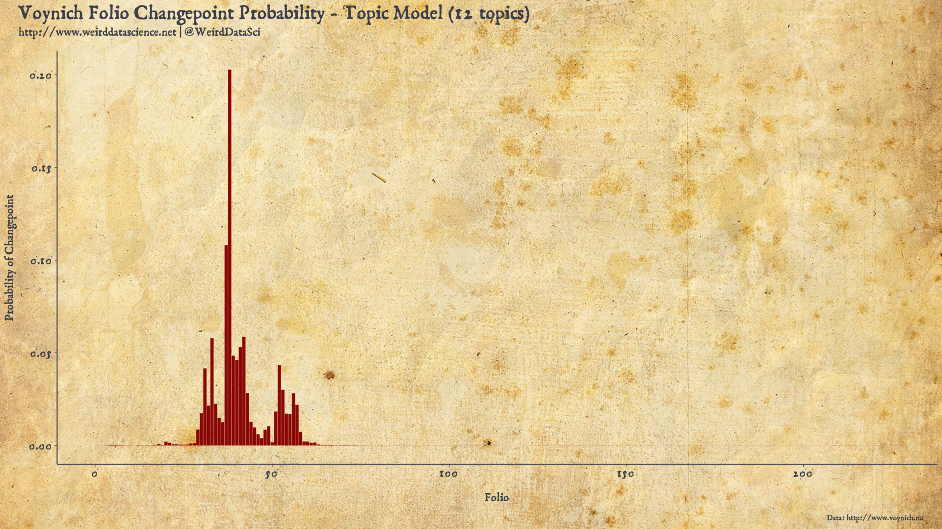
The location suggested for the topic model changepoint are surprisingly close to the results of the changepoint for the frequency counts of short words in the Voynich Manuscript. Whilst the changepoint probabilities are somewhat more diffuse in the topic model analysis, the most significant probability mass is centered around Folio 38, with much lower spikes extending out as far as Folio 55 and Folio 30.
In addition to the mutual support that these two analyses provide, it is notable that the major changpoint identified by both falls directly in the earlier portion of the first, major “herbal” section identified manually by Voynich scholars through inspection of the images accompanying the text. This suggests that that first section, at least in terms of textual content, is not as homogeneous as has previously been suggested. Future scholars investigating the structure of the Voynich Manuscript may therefore wish to direct more attention towards the earlier middle of the herbal section, around folios 30 to 40, to identify what dreadful changes may emerge at that point in the text.
We might naturally, but do not here, extend this analysis by shattering further the smooth unity of the Manuscript according to multiple changepoints. Such an extension is, as intimated in the guide, conceptually simple but computationally burdensome, as it requires recalculation of multiple potential distributions across an ever increasing number of parameters. As such, we leave this analysis, and the means to conduct it more efficiently, for the dim future.
Omnia mutantur, nihil interit
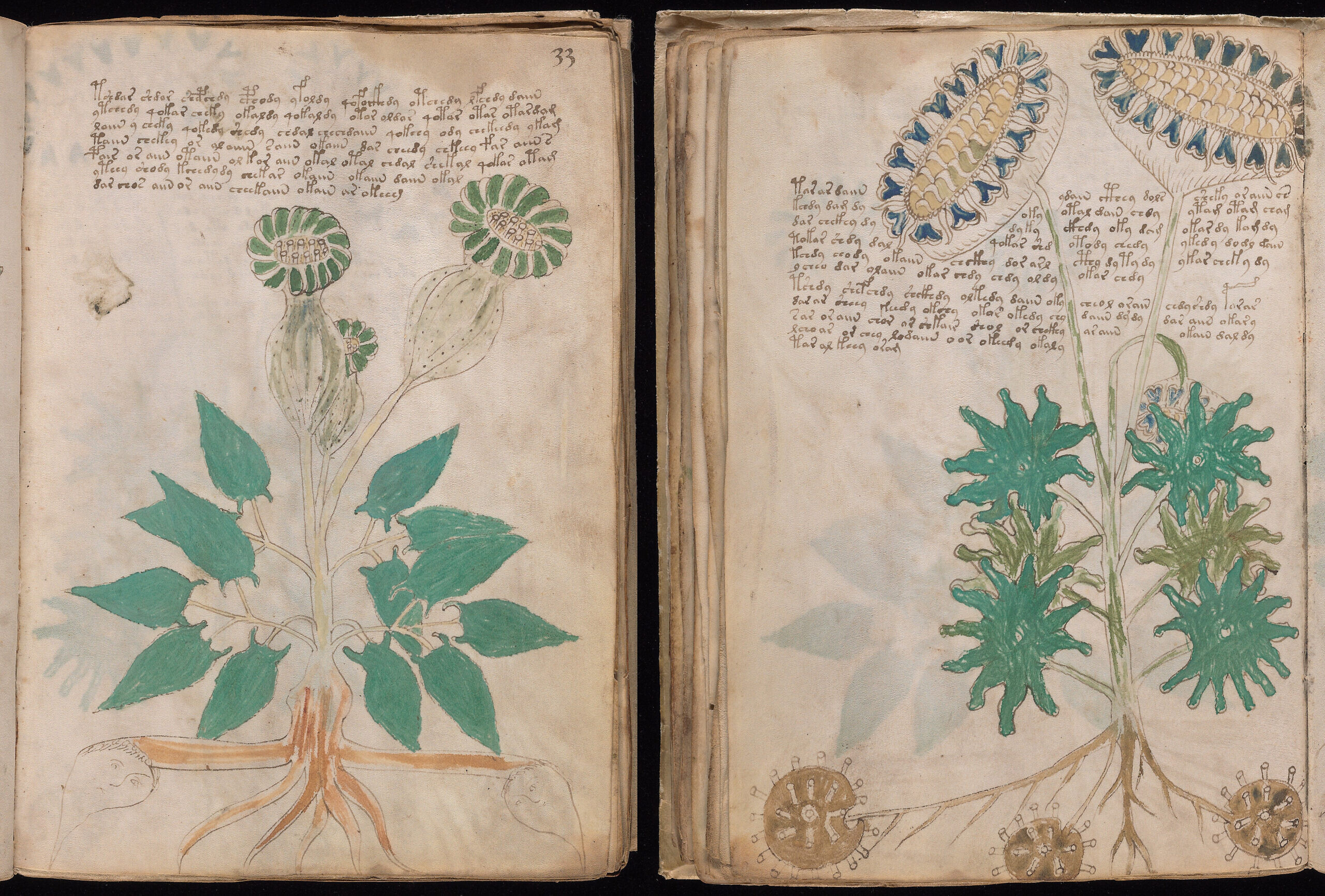
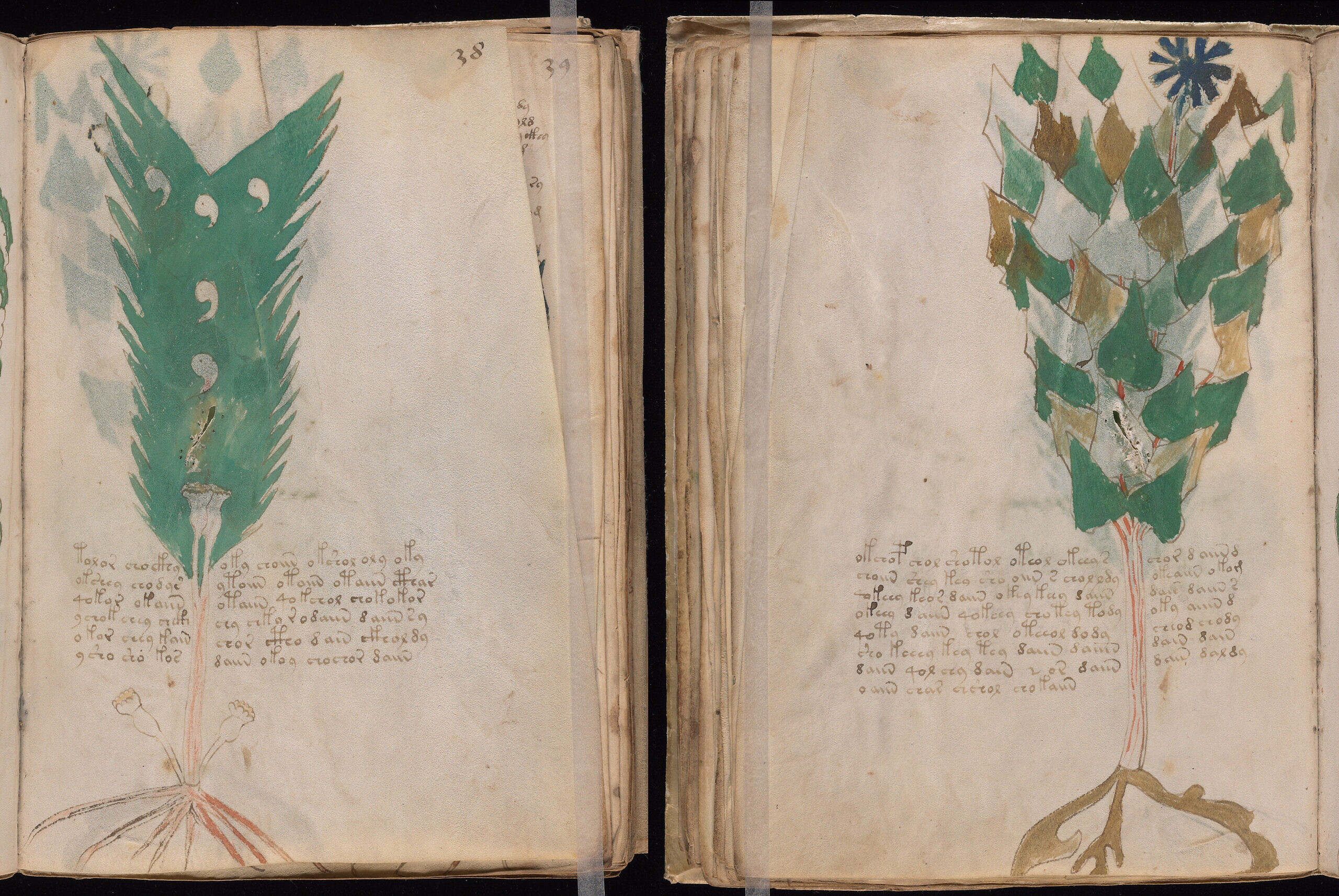
Our analysis has provided us with an abstracted location in the text at which our unsettling suspicions of change lie. The two folios arousing greatest curiosity are therefore Folio 33 and Folio 38, which we present here to reify our horror. It is worth highlighting, however, that the changepoint analysis says nothing specific about these two folios; the model identifies that the inexplicable scrawling prior to the changepoint differs significantly from the maddeningly incomprehensible glyphs following it, nothing more.
Voynich Folio 33Voynich Folio 38
The statistical properties that we have uncovered in the Voynich Manuscript over the past four posts reveal something of its inner structure. It supports, but cannot prove, that the Manuscript is not a hoax, and that it the text is most likely drawn from some natural language.
The changepoint analyses in this post are a powerful tool for identifying evolution and mutation in data, and the demonstrated example of stylometric analysis to Martorel’s Tirant lo Blanc support their use in revealing points of fracture in texts, without reference to the source language.
With specific relevant to the Voynich Manuscript, both the word frequency changepoint and the topic model changepoint suggest that the manscript’s contents shift significantly at some point around Folios 30 to 40. Given the previous assignment of topics based on manual identification of images accompanying the text, this presents a new avenue of investigation for Voynich researchers.
We have resisted that tantalising draw of attempts to translate the Voynich Manuscript. The tools we have applied are more broadly statistical and aim at unveiling structures and revealing patterns in the text; whilst they may provide information towards deciphering the text, that particular conundrum is for the future.
There are, as we would always wish, many avenues left unexplored in this particular labyrinth. The topic model is crude, and more subtle disassemblies could well provide a more refined view. The word frequency patterns support natural language, but we have not made any effort to correlate them with known languages. We have treated words as a unit of analysis, but have not looked in detail at the structure of likely prefixes and suffixes; similar words with differing endings are particularly notable in the topic model, and analysis of these could reveal much more than we have dared to attempt.
There could be much to learn from assessing multiple changepoints in the Manuscript. The presentation of the volume certainly supports its composition of multiple disparate sections; perhaps identifying an inexorable sequence of stylistic shifts could unveil still more of this structure.
For now, however, our meandering journey into the dim twilight of the Voynich Manuscript has drawn to a close, leaving us still searching for illumination in the shadows of this most elegant enigma.

 Tirant lo Blanc Changepoint | (PDF Version)