When working with geo-spatial data in R, I usually use the sf package for manipulating spatial data as Simple Features objects and ggplot2 with geom_sf for visualizing these data. One thing that comes up regularly is “zooming in” on a certain region of interest, i.e. displaying a certain map detail. There are several ways to do so. Three common options are:

• selecting only certain areas of interest from the spatial dataset (e.g. only certain countries / continent(s) / etc.)
• cropping the geometries in the spatial dataset using sf_crop()
• restricting the display window via coord_sf()

I will show the advantages and disadvantages of these options and especially focus on how to zoom in on a certain point of interest at a specific “zoom level”. We will see how to calculate the coordinates of the display window or “bounding box” around this zoom point.

Loading the required libraries and data

We’ll need to load the following packages:

library(ggplot2)
library(sf)
library(rnaturalearth)

Using ne_countries() from the package worldmap, we can get a spatial dataset with the borders of all countries in the world. We load this data as a “simple feature collection” by specifying returnclass = 'sf'. The result is a spatial dataset that can be processed with tools from the sf package.

worldmap <- ne_countries(scale = 'medium', type = 'map_units',
                         returnclass = 'sf')
# have a look at these two columns only
head(worldmap[c('name', 'continent')])

Simple feature collection with 6 features and 2 fields
geometry type: MULTIPOLYGON
dimension: XY
bbox: xmin: -180 ymin: -18.28799 xmax: 180 ymax: 83.23324
epsg (SRID): 4326
proj4string: +proj=longlat +datum=WGS84 +no_defs
name continent geometry
0 Fiji Oceania MULTIPOLYGON (((180 -16.067...
1 Tanzania Africa MULTIPOLYGON (((33.90371 -0...
2 W. Sahara Africa MULTIPOLYGON (((-8.66559 27...
3 Canada North America MULTIPOLYGON (((-122.84 49,...
4 United States of America North America MULTIPOLYGON (((-122.84 49,...
5 Kazakhstan Asia MULTIPOLYGON (((87.35997 49...

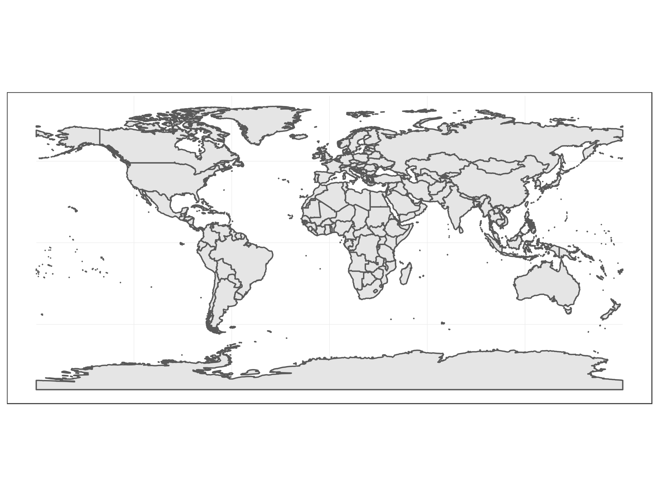
We see that we have a spatial dataset consisting of several attributes (only name and continent are shown above) for each spatial feature which is stored in the geometry column. The header above the table displays further information such as the coordinate reference system (CRS) which will be important later. For now, it is important to know that the coordinates in the plot are longitude / latitude coordinates in degrees in a CRS called WGS84. The longitude reaches from -180° (180° west of the meridian) to +180° (180° east of the meridian). The latitude reaches from -90° (90° south of the equator) to +90° (90° north of the equator).

Let’s plot this data to confirm what we have:

ggplot() + geom_sf(data = worldmap) + theme_bw()

Selecting certain areas of interest from a spatial dataset

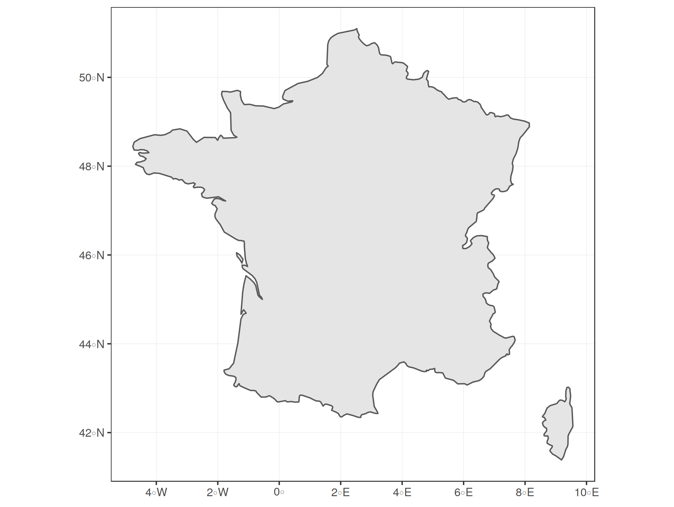
This is quite straight forward: We can plot a subset of a larger spatial dataset and then ggplot2 automatically sets the display window accordingly, so that it only includes the selected geometries. Let’s select and plot France only:

france <- worldmap[worldmap$name == 'France',]
ggplot() + geom_sf(data = france) + theme_bw()

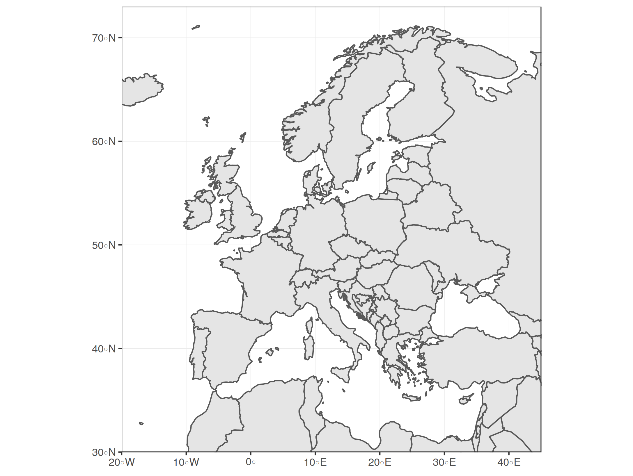
Let’s try to select and plot all countries from Europe:

europe <- worldmap[worldmap$continent == 'Europe',]
ggplot() + geom_sf(data = europe) + theme_bw()

Well, this is probably not the section that you want to display when you want to make a plot of Europe. It includes whole Russia (since its continent attribute is set to "Europe") which makes the plot span the whole northern globe. At the same time, nearby countries such as Turkey or countries from northern Africa are missing, which you might want to include to show “context” around your region of interest.

Cropping geometries in the spatial dataset or restricting the display window

To fix this, you may crop the geometries in your spatial dataset as if you took a knife a sliced through the shapes on the map to take out a rectangular region of interest. The alternative would be to restrict the display window of your plot, which is like taking the map and folding it so that you only see the region of interest. The rest of the map still exists, you just don’t see it.

So both approaches are quite similar, only that the first actually changes the data by cutting the geometries, whereas the latter only “zooms” to a detail but keeps the underlying data untouched.

Let’s try out the cropping method first, which can be done with sf_crop(). It works by passing the spatial dataset (the whole worldmap dataset in our case) and specifying a rectangular region which we’d like to cut. Our coordinates are specified as longitude / latitude in degrees, as mentioned initially. We set the minimum longitude (i.e. the left border of the crop area) as xmin and the maximum longitude (i.e. right border) as xmax. The minimum / maximum latitude (i.e. lower and upper border) are set analogously as ymin and ymax. For a cropping area of Europe, we can set the longitude range to be in [-20, 45] and latitude range to be in [30, 73]:

europe_cropped <- st_crop(worldmap, xmin = -20, xmax = 45,
                                    ymin = 30, ymax = 73)
ggplot() + geom_sf(data = europe_cropped) + theme_bw()

You can see that the shapes were actually cropped at the specified ranges when you look at the gaps near the plot margins. If you want to remove these gaps, you can add + coord_sf(expand = FALSE) to the plot.

We can also see that we now have clipped shapes when we project them to a different CRS. We can see that in the default projection that is used by ggplot2, the grid of longitudes and latitudes, which is called graticule, is made of perpendicular lines (displayed as light gray lines). When we use a Mollweide projection, which is a “pseudo-cylindrical” projection, we see how the clipped shapes are warped along the meridians, which do not run in parallel in this projection but converge to the polar ends of the prime meridian:

Restricting the display window for plotting achieves a very similar result, only that we don’t need to modify the spatial dataset. We can use coord_sf() to specify a range of longitudes (xlim vector with minimum and maximum) and latitudes (ylim vector) to display, similar to as we did it for st_crop():

ggplot() + geom_sf(data = worldmap) +
    coord_sf(xlim = c(-20, 45), ylim = c(30, 73), expand = FALSE) +
    theme_bw()

You see that the result is very similar, but we use the whole worldmap dataset without cropping it. Notice that I used expand = FALSE which removes the padding around the limits of the display window (this is what produced the “gaps” at the plot margins before).

Now what if we wanted to use the Mollweide projection again as target projection for this section? Let’s try:

ggplot() + geom_sf(data = worldmap) +
    coord_sf(crs = st_crs('+proj=moll'),
             xlim = c(-20, 45), ylim = c(30, 73),
             expand = FALSE) +
    theme_bw()

What happened here? The problem is that we specified xlim and ylim as WGS84 coordinates (longitude / latitude in degrees) but coord_sf needs these coordinates to be in the same CRS as the target projection, which is the Mollweide projection in our case. Mollweide uses meters as unit, so we actually specified a range of -20m to 45m on the x-scale and 30m to 73m on the y-scale, which is a really tiny patch near the center of projection.

So in order to fix that, we’d need to transform the coordinates of the display window to the target CRS first. First, let’s get a visual overview on what we want to do:

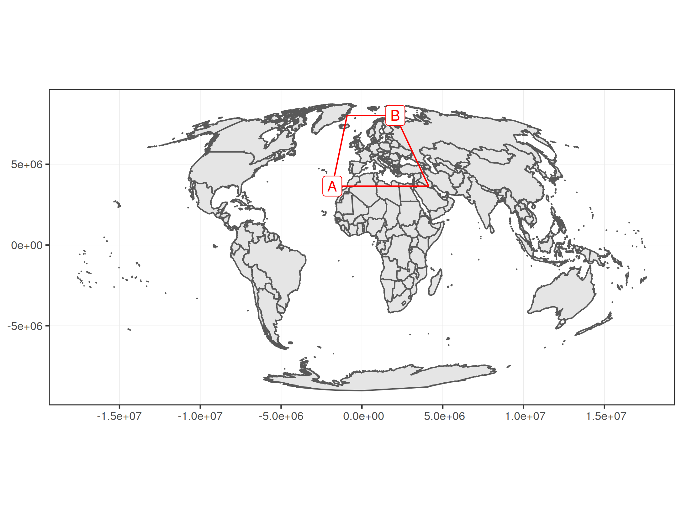
What we see is the whole worldmap dataset projected to our target CRS (standard Mollweide projection). There are two points, A = (-20°, 30°) and B = (45°, 73°), which define our display window, highlighted with red lines. The display window is a trapezoid because the originally rectangular display window defined by longitude / latitude coordinates is warped along the meridians, just as our cropped shape of Europe before. When you have a look at the axes, you’ll see that there are no degrees displayed here anymore. Instead, the graticule shows the target CRS, which has the unit meters (this is why the numbers on the axes are so large). Our corner points of the display window A and B must be converted to this CRS, too, and we can do that as follows:

At first, we set the target CRS and transform the whole worldmap dataset to that CRS.

target_crs <- '+proj=moll'
worldmap_trans <- st_transform(worldmap, crs = target_crs)

Next, we specify the display window in WGS84 coordinates as longitude / latitude degrees. We only specify the bottom left and top right corners (points A and B). The CRS is set to WGS84 by using the EPSG code 4236.

disp_win_wgs84 <- st_sfc(st_point(c(-20, 30)), st_point(c(45, 73)),
                         crs = 4326)
disp_win_wgs84

Geometry set for 2 features
geometry type:  POINT
dimension:      XY
bbox:           xmin: -20 ymin: 30 xmax: 45 ymax: 73
epsg (SRID):    4326
proj4string:    +proj=longlat +datum=WGS84 +no_defs
POINT (-20 30)
POINT (45 73)

These coordinates can be transformed to our target CRS via st_transform.

disp_win_trans <- st_transform(disp_win_wgs84, crs = target_crs)
disp_win_trans

Geometry set for 2 features
geometry type:  POINT
dimension:      XY
bbox:           xmin: -1833617 ymin: 3643854 xmax: 2065900 ymax: 8018072
epsg (SRID):    NA
proj4string:    +proj=moll +lon_0=0 +x_0=0 +y_0=0 +ellps=WGS84 +units=m +no_defs
POINT (-1833617 3643854)
POINT (2065900 8018072)

We can extract the coordinates from these points and pass them as limits for the x and y scale respectively. Note also that I set datum = target_crs which makes sure that the graticule is displayed in the target CRS. Otherwise ggplot2 by default displays a WGS84 graticule.

disp_win_coord <- st_coordinates(disp_win_trans)

ggplot() + geom_sf(data = worldmap_trans) +
    coord_sf(xlim = disp_win_coord[,'X'], ylim = disp_win_coord[,'Y'],
             datum = target_crs, expand = FALSE) +
    theme_bw()

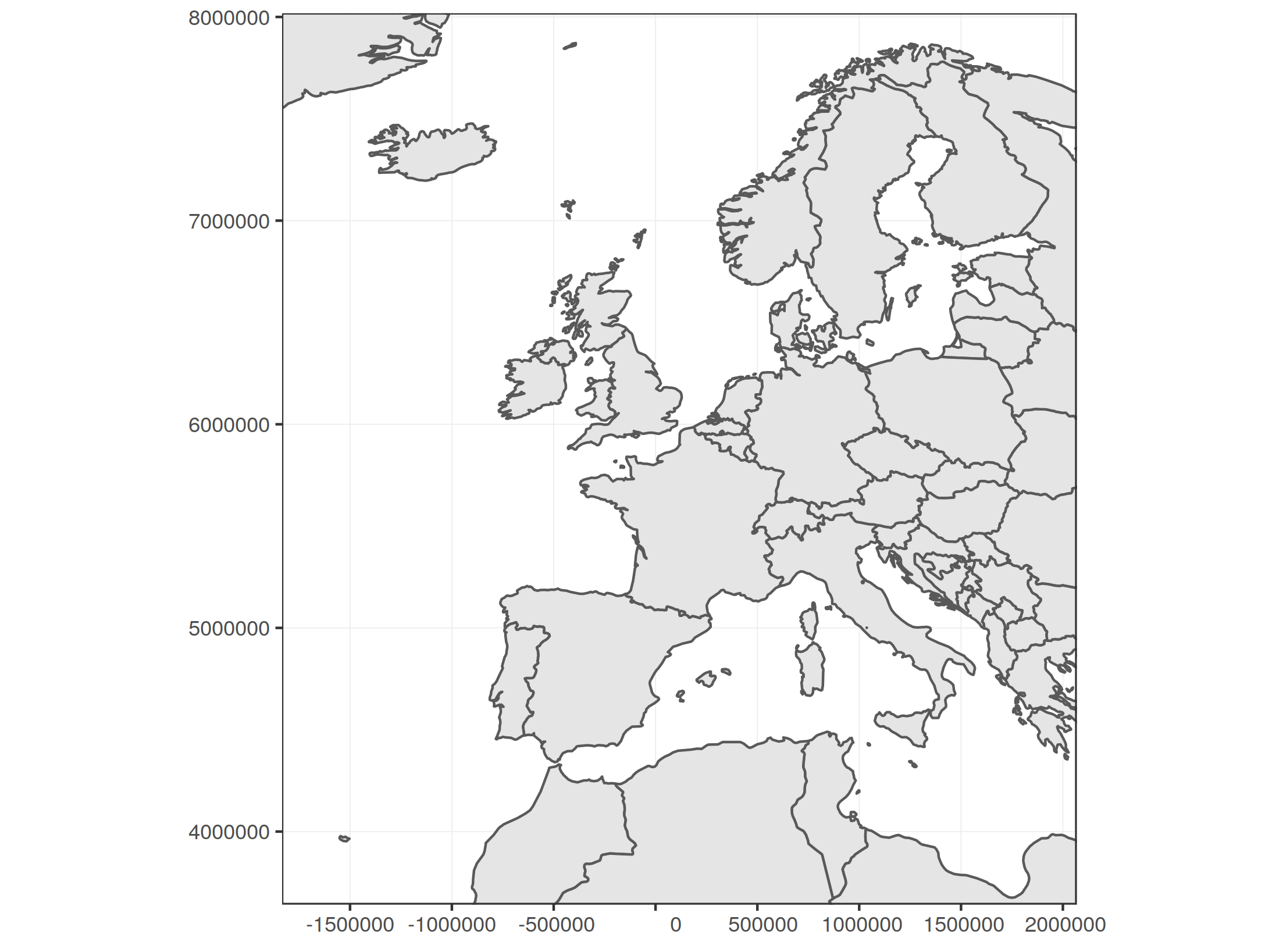
This works, but if you look closely, you’ll notice that the display window is slightly different than the one specified in WGS84 coordinates before (the red trapezoid). For example, Turkey is completely missing. This is because the coordinates describe the rectangle between A and B in Mollweide projection, and not the red trapezoid that comes from the original projection.

Calculating the display window for given a center point and zoom level

Instead of specifying a rectangular region of interest, I found it more comfortable to set a center point of interest and specify a “zoom level” which specifies how much area around this spot should be displayed.

I oriented myself on how zoom levels are defined for OpenStreetMap: A level of zero shows the whole world. A level of 1 shows a quarter of the world map. A level of two shows 1/16th of the world map and so on. This goes up to a zoom level of 19. So if z is the zoom level, we see a region that covers 1/4^z of the world. This means the range on the longitude axis that is displayed is 360°/2^z (because the longitude spans the full horizontal circle around the world from -180° to +180°) and the range on the latitude axis is 180°/2^z (latitude spans the half vertical circle from -90° to +90°).

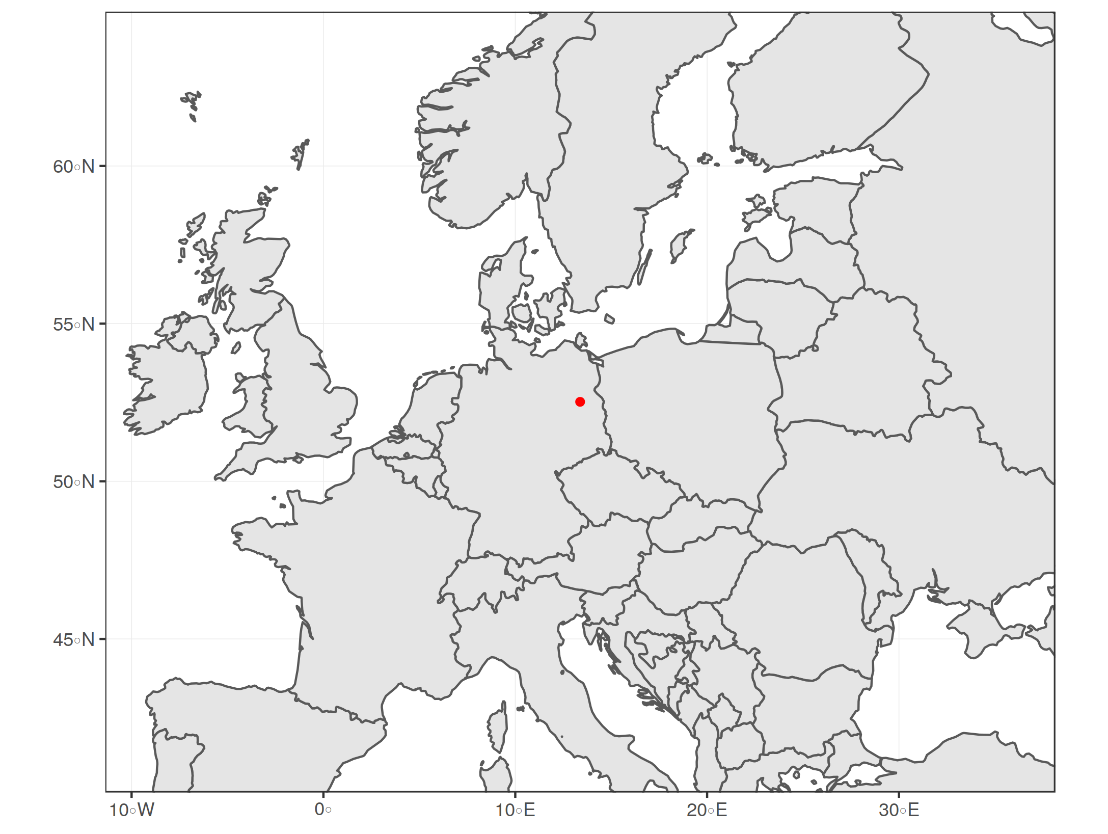
Let’s set a center point zoom_to, a zoom_level and calculate the ranges for longitude and latitude (lon_span and lat_span).

zoom_to <- c(13.38, 52.52)  # Berlin

zoom_level <- 3

lon_span <- 360 / 2^zoom_level
lat_span <- 180 / 2^zoom_level

Now we can calculate the longitude and latitude ranges for the the display window by subtracting/adding the half of the above ranges from/to the zoom center coordinates respectively.

lon_bounds <- c(zoom_to[1] - lon_span / 2, zoom_to[1] + lon_span / 2)
lat_bounds <- c(zoom_to[2] - lat_span / 2, zoom_to[2] + lat_span / 2)

We can now plot the map with the specified display window for zoom level 3, highlighting the zoom center as red dot:

ggplot() + geom_sf(data = worldmap) +
    geom_sf(data = st_sfc(st_point(zoom_to), crs = 4326),
            color = 'red') +
    coord_sf(xlim = lon_bounds, ylim = lat_bounds) + theme_bw()

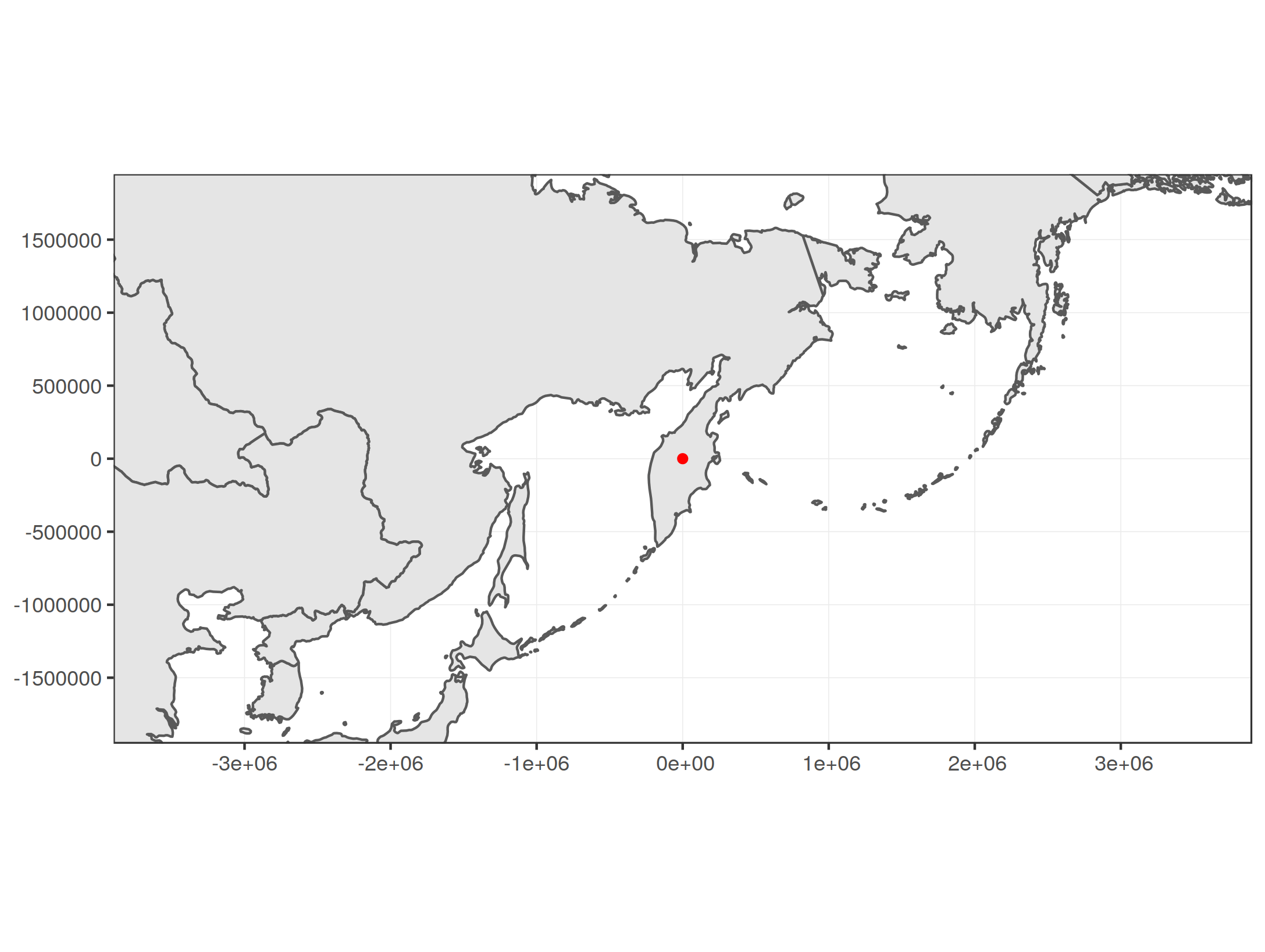
So this works quite good when using the default projection and WGS84 coordinates. How about another projection? Let’s put Kamchatka at the center of our map, set a zoom level, and use a Lambert azimuthal equal-area projection (LAEA) centered at our zoom point:

zoom_to <- c(159.21, 56.41)  # ~ center of Kamchatka
zoom_level <- 2.5

# Lambert azimuthal equal-area projection around center of interest
target_crs <- sprintf('+proj=laea +lon_0=%f +lat_0=%f',
                      zoom_to[1], zoom_to[2])

When we worked with WGS84 coordinates before, we calculated the displayed range of longitude and latitude at a given zoom level z in degrees by dividing the full circle for the longitude (360°) by 2^z and the half circle (180°) for the latitude in the same way. A LAEA projection uses meters as unit instead of degrees, so instead of dividing a circle of 360°, we divide the full circumference of the Earth in meters, which is about C = 40,075,016m, by 2^z to get the display range for the x-axis (corresponding to longitude range before). Similar as before, we use the half circumference (assuming that the Earth is a perfect sphere, which she is not) for the displayed range on the y-axis, so we get C / 2^(z+1).

C <- 40075016.686   # ~ circumference of Earth in meters
x_span <- C / 2^zoom_level
y_span <- C / 2^(zoom_level+1)

We can now calculate the lower left and upper right corner of our display window as before, by subtracting/adding half of x_span and y_span from/to the zoom center coordinate as before. But of course, the zoom center has to be converted to the target CRS, too. We put the zoom point at the center of the projection, so in this special case we already know that it is at (0m, 0m) in the target CRS. Anyway I will provide a, because when you use a standardized CRS with EPSG code, your zoom point probably won’t be the center of projection:

zoom_to_xy <- st_transform(st_sfc(st_point(zoom_to), crs = 4326),
                           crs = target_crs)
zoom_to_xy

Geometry set for 1 feature
geometry type:  POINT
dimension:      XY
bbox:           xmin: 1.570701e-09 ymin: 7.070809e-10 xmax: 1.570701e-09 ymax: 7.070809e-10
epsg (SRID):    NA
proj4string:    +proj=laea +lat_0=56.41 +lon_0=159.21 +x_0=0 +y_0=0 +ellps=WGS84 +units=m +no_defs
POINT (1.570701e-09 7.070809e-10)

Rounding errors aside, this confirms that the zoom point is at the center of projection. We can now calculate the display window coordinates as stated before¹:

disp_window <- st_sfc(
    st_point(st_coordinates(zoom_to_xy - c(x_span / 2, y_span / 2))),
    st_point(st_coordinates(zoom_to_xy + c(x_span / 2, y_span / 2))),
    crs = target_crs
)

And now passing the display window coordinates to coord_sf, we can plot the result:

 ggplot() + geom_sf(data = worldmap) +
    geom_sf(data = zoom_to_xy, color = 'red') +
    coord_sf(xlim = st_coordinates(disp_window)[,'X'],
             ylim = st_coordinates(disp_window)[,'Y'],
             crs = target_crs, datum = target_crs) +
    theme_bw()

You can try this out with different zoom levels, zoom center points and projections. Note that some combinations of zoom levels and projections will cause projection errors, since some projection are only specified within certain bounds and not for the whole world. I put the full R script in this gist.

¹ Again, we could simplify this in the special case where the zoom point is the center of projection. Also note that I had to wrap each coordinate in st_point(st_coordinates(...)), which seems redundant but was the only way to get it working. It looks like the sf objects lose the CRS information when applying vector operations to them.