Introduction

During my Master’s of Data Science studies at Faculty of Economics University of Warsaw, at Unsupervised Learning Classes I got a task to write a paper about Principal Component Analysis. The goal of this method is to “identify patterns in data and express the data in such a way as to highlight their similarities and differences” (Smith, 2002). So, imagine, you have a huge dataset with hundreds of variables, which makes it a really tough thing to understand and analyze. That is where PCA comes with help. The method, using set of different matrix operations, verifies dependencies between variables. It checks whether few variables could actually be described by one, common variable or it also finds those features, which are rather not important to get a proper understanding of the data we have.  In other words it gets the most important information included in dataset. For a better understanding of PCA I highly recommend this topic https://stats.stackexchange.com/questions/2691/making-sense-of-principal-component-analysis-eigenvectors-eigenvalues.
What is important about PCA is that with reducing the number of irrelevant or less important variables we can get a much lighter new data set, which can describe most of the patterns the original data did. Of course, the more we simplify our data with PCA the less precise perspective we can get.

After this short overview I am able to explain the aim of this paper. The ability of PCA to simplify a data made it a popular tool in area of Image-Compression. Why is so? However insensitively it might sound, the digital image is just a 2D array (or arrays in case of color pictures) of pixels with different parameters. It is said that using PCA it is possible to reduce the size of the photo in such a way that the change in quality would be marginal. How does the theorem work in reality? I try to verify that in next chapters using R codes.

This post is divided into the following chapters:

• Methodology and data (images)
• R codes
• Comparison of the results
• Conclusion

1. Methodology and data (images)

To conduct my analysis I use 2 different R codes and 2 images (black and white, color). Also, there is a necessity to compare the results of different approaches, so measures of image compression quality are also described in this chapter. But at first I include my PC’s specification. It is because some operations I conducted during the analysis made my computer to work really hard. After running few of the codes the only thing which asured me that my PC did not crash was that I was able to move a cursor.

1.1. PC specification

• Windows Version: Windows 7 Professional 64 bits
• Processor: Intel Core i5-2400 3.1 GHz
• RAM: 12 GB
• Graphics Card: NVIDIA GeForce GTX 660

1.2. Images

1.2.1. Image A (black and white)

link: https://pixabay.com/pl/kapsztad-dzielnicy-camps-bay-2847751/

The picture is surely black and white, however when you read it into R, it occurs that the program interprets it as the color one (with RGB scale). Here is the code to turn color picture into gray-scaled one:

library(jpeg)

photo <- readJPEG("yourphoto.jpg")

photo <- photo[,,1]+photo[,,2]+photo[,,3]

photo <- photo/max(photo)

writeJPEG(photo, "b&w_photo.jpg")

1.2.2. Image B (color)

link: http://www.effigis.com/wp-content/uploads/2015/02/Airbus_Pleiades_50cm_8bit_RGB_Yogyakarta.jpg

1.3. Codes

1.3.1. Code 1

It is my own code, which bases on the theorem of Covariance Matrix Method described in this article:

https://www.researchgate.net/publication/309165405_Principal_component_analysis_-_a_tutorial

Here are the algorithms which Code 1 is built on. It is hard to say why author created two algorithms for basicaly the same operation. Anyway, if you would like to implement that, I recommend to stick to algorithm 1 and at the end go to point 6 from algorithm 4. Also, if you want to understand whole process in a better way, in the paper I attached there is a really good example of Algorithm 1 usage in chapter 3.1.

What should be said about Code 1 is that it is applicable rather only to gray-scaled images. The black and white images are read by computer as one matrix, while color images are converted into 3 matrixes, with every matrix for one scale (R and G and B) of colors from RGB. To use Code 1 for color image – compression the provided code should be replicated in loops for every matrix. It takes a lot of memory. It was surely too much for my PC.

1.3.2. Code 2

This code was written by Aaron Schlegel and is available here: http://www.r-bloggers.com/image-compression-with-principal-component-analysis/

In the version provided on the blog it is applicable to color images. However, in the next chapter I present a little modification of this code which works for gray-scaled pictures. It is important to indicate that although this code works for color images, it can be a serious challenge for your computer. When I made a first try with it, I used 50 mbs image to get converted. After running the code I had enough time to clean my kitchen, cause all processing took about 30 minutes and it was consuming all of my PC’s resources.

1.4. Methodology summary

Now, when I have pointed out all the codes’ limitations I can describe the final methodology. I carry out 3 tests.

• Test 1 – Code 1 + Image A
• Test 2 – Code 2 + Image A
• Test 3 – Code 2 + Image B

In the next chapter codes for all 3 tests are provided with some additional comments.

2. R codes

2.1. Test 1

library(jpeg)

photo <- readJPEG("photo.jpg")

####### step 2 and 3 Algorithm 1 #######
mean <- rowMeans(photo)
D <- sweep(photo, 1, rowMeans(photo))

####### step 4 Algorithm 1 #######
covix <- 1/(ncol(photo)-1) * D %*% t(D)


####### step 5, 6, 6 Algorithm 1 #######
eigenn <- eigen(covix)
eigen_vectors <- eigenn$vectors


####### Defining number of PCs we want to use #######
PCs <- c(round(0.1 * nrow(photo)), round(0.2 * nrow(photo)),
         round(0.3 * nrow(photo)), round(0.4 * nrow(photo)),
         round(0.5 * nrow(photo)), round(0.6 * nrow(photo)),
         round(0.7 * nrow(photo)), round(0.8 * nrow(photo)), 
         round(0.9 * nrow(photo)))


for (i in PCs){
  ####### Step 7 Algorithm 1 #######
  W <- eigen_vectors[,1:i]
  W <- as.matrix(W)
  
  ####### Step 8 Algorithm 1 #######
  Y <- t(W) %*% D

  ####### Step 6 Algorithm 2 #######
  I = W %*% Y
  I <- sweep(I, 1, mean, "+")
  
  ####### Saving the image #######
  writeJPEG(I, paste('photo_compressed_', i , '_components.jpg', sep = ''))
}

What should be said about this code is:

• In step 4 we calculate covariance matrix, however we can’t use R built in function cov(), because it doesn’t return the covariance matrix which can be used in the analysis. (Look equation 12, Algorithm 1, 1.3.1)
• In step 5, 6, 7, luckily, function eigen() does all 3 steps of the Algorithm 1 (look 1.3.1) at once.

Pictures are still to big to upload them here. Few of them are available at:

https://drive.google.com/drive/folders/1MBW7Mcvg1JCDmzp0ob3ZUuziNNqQEhpj?usp=sharing

I discuss the size of obtained compressed images and other statistics in chapter 3.

2.2. Test 2

library(jpeg)

####### reading an image #######
photo <- readJPEG("photo.jpg")

####### introducing PCA method #######
photo.pca <- prcomp(photo, center = F)

####### Image compression with different values of PCs #######
PCs <- c(round(0.1 * nrow(photo)), round(0.2 * nrow(photo)),
         round(0.3 * nrow(photo)), round(0.4 * nrow(photo)),
         round(0.5 * nrow(photo)), round(0.6 * nrow(photo)),
         round(0.7 * nrow(photo)), round(0.8 * nrow(photo)), 
         round(0.9 * nrow(photo)))

for (i in PCs){
    pca.img <- photo.pca$x[,1:i] %*% t(photo.pca$rotation[,1:i])
    writeJPEG(pca.img, paste("photo_", i, "_compontents.jpg", sep = ""))
}

The code here is much simpler than in Test 1. Prcomp function covers most of the operations, which in Test 1 were done separately. It is crucial to indicate that function prcomp uses Singular Value Decomposition method which is an alternative to Covariance Matrix Method from Test 1. But, to be honest, independently from the method, neither test 1 nor test 2 give satisfacionary results. You will find out more about that in chapter 3.

The compressed pictures (few of them) from test 2 are available here:

https://drive.google.com/drive/folders/1xSJ3uYzRNbs4qat0couiQ-1e22mh8QQD?usp=sharing

2.3. Test 3

library(jpeg)

####### read photo #######
photo <- readJPEG("your_photo.jpg")

####### Creating separated matrix for every RGB color scale #######
r <- photo[,,1]
g <- photo[,,2]
b <- photo[,,3]

####### Introducing PCA method #######
r.pca <- prcomp(r, center = F)
g.pca <- prcomp(g, center = F)
b.pca <- prcomp(b, center = F)

rgb.pca <- list(r.pca, g.pca, b.pca)



for (i in seq.int(3, round(nrow(photo) - 10), length.out = 10)) {
  pca.img <- sapply(rgb.pca, function(j) {
    compressed.img <- j$x[,1:i] %*% t(j$rotation[,1:i])
  }, simplify = 'array')
  writeJPEG(pca.img, paste('photo_', round(i,0), '_components.jpg', sep = ''))
}

Test 3 is the only one from these conducted in this post which gives really good results. Here are few images compressed with test 3:

https://drive.google.com/drive/folders/18Wr_rcdmXGiMi676Q_MINkR3EyVSTj2p?usp=sharingh

3. Comparison of the results

3.1. Measures

To compare the results of image compression 4 measures were introduced, labeled as follows:

• Photo_file_size
• Photo_PCs_vs_MSE
• Photo_PCs_vs_PSNR
• Photo_PCs_vs_file_size

It has not been said before, but it is important to know that the maximum number of PCs (Principal Components) is the number of rows of the original photo’s matrix. Below there is a description of what measures listed above stand for and what they are based on.

3.1.1. Photo_file_size

That is the most important of our measures. The aim of compression is to reduce size of the image. So to know how efficient were our actions we need to know what is the size (in this case sizes, cause for every test many options were verified) of a compressed image.

3.1.2. Photo_PCs_vs_MSE

MSE – Mean Squared Error is the measure of difference between the original image and compressed one. The lower is the number of PCs the more simplified is the image. In this work I calculated this value using function mse from Metric package.

3.1.3. Photo_PCs_vs_PSNR

PSNR – Peak Signal to Noise Ratio is “Most commonly used measure of the quality of photo compression. The signal in this case is the original data and the noise is the error introduced by compression. (…) It is an approximation to human perception of compressed image quality. Although the higher PSNR generally indicates that the reconstruction is of  higher quality, in some cases it may not” (Singh and Kumar, 2006). Below there is an equation for PSNR.

3.1.4. Photo_PCs_vs_file_size

This measure just checks the file size of all new images depending on the number of PCs which were used to obtain them.  

3.2. Results

The code to get measures and visualizations of them is, luckily, common for all tests. That is how it looks like:

library(Metrics)
library(magicfor)
library(ggplot2)
library(gridExtra)
library(grid)

PCs <- c(all PCs you used in previous part of coding)
####### getting file size #######

magic_for()
for (i in PCs){
  size <- file.size(paste('photo_compressed_', i, '_components.jpg', sep = ''))
  put(size/1000000)
}  
file_size <- magic_result_as_vector()
file_size_orginal <- file.size("photo.jpg")/1000000
file_size_data <- data.frame("Number_of_PCs" = 
                               c("Original_Photo", PCs), 
                             "MBs" = c(file_size_orginal, file_size))

file_size_data$Number_of_PCs <- factor(file_size_data$Number_of_PCs, 
                                       levels = file_size_data$Number_of_PCs
                                       [order(file_size_data$MBs)])


####### Getting mse values for next levels of PCs #######

magic_for()
for (i in PCs){
  photo_mse <- readJPEG(paste('photo_compressed_', i, '_components.jpg', sep = ''))
  mse_val <- mse(photo, photo_mse)
  put(mse_val)
} 
mse_result <- magic_result_as_vector()


####### PSNR calculation #######

magic_for()
for (i in PCs){
  photo_PSNR <- readJPEG(paste('photo_compressed_', i, '_components.jpg', sep = ''))
  MAX <- max(photo_PSNR)
  put(MAX)
} 
MAX <- magic_result_as_vector()


####### Creating Data Frame for plots #######

df <- data.frame("Number_of_PCs" = PCs, "MSE" = mse_result, "File_size" = file_size, "MAX" = MAX)
df[,"PNSR"] <- 10*log10(df$MAX^2/df$MSE)


####### Getting plots #######

photo_PCs_vs_MSE <- ggplot(df, aes(x = Number_of_PCs, y = MSE)) + geom_point() + geom_line(color = "red")
photo_PCs_vs_File_size <- ggplot(df, aes(x = Number_of_PCs, y = File_size)) + geom_point() + geom_line(color = "orange")
photo_PCs_vs_PSNR <- ggplot(df, aes(x = Number_of_PCs, y = PNSR)) + geom_point() + geom_line(color = "green")
photo_file_size_barplot <- ggplot(file_size_data, aes(x = Number_of_PCs, y = MBs)) + geom_bar(stat = "identity")

combined <- grid.arrange(photo_PCs_vs_MSE, photo_PCs_vs_PSNR, photo_PCs_vs_File_size, nrow = 3, 
                         top = textGrob("Title",gp=gpar(fontsize=20,font=3)))

####### Saving plots #######

ggsave("photo_PCs_vs_MSE.jpg", photo_PCs_vs_MSE, device = "jpeg")
ggsave("photo_PCs_vs_File_size.jpg", photo_PCs_vs_File_size, device = "jpeg")
ggsave("photo_PCs_vs_PSNR.jpg", photo_PCs_vs_PSNR, device = "jpeg")
ggsave("photo_file_size_barplot.jpg", photo_file_size_barplot, device = "jpeg")
ggsave("photo_combined.jpg", combined, device = "jpeg")

3.2.1. Test 1 vs Test 2

Test 1 and Test 2 worked with the same black and white photo but with different codes, so it is interesting to verify, which of the codes performed better.

As it was mentioned before, to check whether the compression was successful it is essential to compare file size between original and every of the compressed images. Here it is how it looks like:

Actually, we find out that both codes performed approximately the same. And it was not a good performance, cause in both cases most of the compressed images have a bigger file size than the original one, so it is some kind of anti-compression . For both tests the file size was lower only for the images compressed with 3 and 567(10% of all) PCs. And, well, 3 PCs compressed image’s size is more than 4 times smaller than the original one, but it does not look as original photo at all. With 567 PCs we get an image which is about 1.5 mb smaller than original one. It is better than in the first case, cause the compressed image is similar to the original one, but the quality is obviously worse. So it is up to you to answer yourself is it worth to save 1.5 mb to get much worse looking image (maybe with a huge photo gallery it would make sense).

What about other measures?

For PSNR and MSE we find out, what is rather obvious, that the more PCs we used to conduct the compression the better those stats are. However, having in mind that most of the compressions gave us heavier files than the original one, analyzing this stats does not have much sense.

What is maybe more interesting is that the relation between PCs used for compression and file_size is not linear. In both cases the heaviest is the file with 1702 components (30% of all). It is 1 mb heavier than original one.    

So all measures were verified and what do we know after that? Test 1 and test 2 use different codes based on 2 methods, respectively: Covariance Matrix Method and Singular Value Decomposition. But, what made me a little bit disappointed, independently from the method, both codes provided us with really poor results, reducing the file size only in 2 cases and even increasing it in 8 other situations. I checked this observation for few different original images and in all cases it worked similarly badly. But I have a good news. Although, the conversion for black and white image is not satisfying, it surely is for a color one. Here it comes.

3.2.2. Test 3

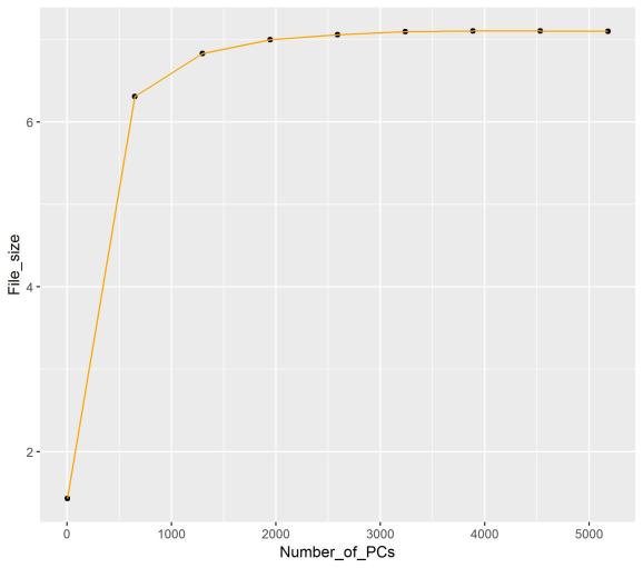
As I spoilered at the end of previous chapter, compression of color image went in really satisfying way. All results are shown below. Let’s begin with file size comparison:

In all cases file size reduction was really significant. The one with 3 components is 40 times smaller, and one with 5182 components (88 % of all) is 5.7 times smaller  . What is important we not only get the much lighter image but it is really hard to spot the difference in quality between the 5182 PCs image and the original one.

Here are other measures:

What might be interesting about MSE and PSNR is to spot the pattern, that the more PCs were used to conduct a compression the less is the change in quality measures. So at the beginning going from 3 (close to 0% of all PCs) to 650 (which is about 10%) gives us a huge change in MSE and PSNR stats. But when you will take a look at the difference for both measures between 4534 (close to 80%) and 5182 PCs (about 90% of all), you will see that the change in values is marginal. This observation coincides with what one can just conclude from looking at compressed images. The compressed image with 3 components looks nothing like the original picture, but the one with 650 PCs is exactly the original image, just in worse quality. So we have a huge change here. But trying to find differences between compressed images with 4534 PCs and 5182 PCs is a really difficult task.

Anyway, what should be highlighted after describing the results of test 3 is that it gave us really effective compression. So this method and code is not only useful for writing a paper for your classes, but it can be also used for actual needs.

4. Conclusion

The aim of the whole analysis was to conduct PCA based image – compression with R. The study was done with two images: black and white and color and two codes basing on slightly different methods: Covariance Matrix Method and Singular Value Decomposition.

Covariance Matrix Method code, in this paper labeled as Code 1, was applied only to black and white image, because of its heavy memory usage. Singular Value Decomposition code, labeled as Code 2, was used both for: black and white image and the color one.

Both Code 1 and Code 2 failed to provide satisfying compressions for black and white image. Although, in some cases they reduced file size it all came with a huge quality loss.

Luckily, for the compression of color image, Code 2 had an outstanding performance. It significantly reduced file size for all PC levels which were used. And it all happened with a really low loss in photo quality.

References

Airbus. (2015). Yogyakarta Airport, Indonesia. Retrieved from: http://www.effigis.com/wp-content/uploads/2015/02/Airbus_Pleiades_50cm_8bit_RGB_Yogyakarta.jpg
Amoeba. (2010). Making sense of principal component analysis, eigenvectors & eigenvalues. Retrieved from: https://stats.stackexchange.com/questions/2691/making-sense-of-principal-component-analysis-eigenvectors-eigenvalues
Mawe001. (2016). Cape Town Camps Bay District. Retrieved from: https://pixabay.com/pl/kapsztad-dzielnicy-camps-bay-2847751/#comments
Schlegel, A. (2017). Image Compression with Principal Component Analysis. Retrieved from: http://www.r-bloggers.com/image-compression-with-principal-component-analysis/
Singh, A. and Kumar, S. (2016). An overview of PCA and jpeg image compression scheme. International Journal of Electrical and Electronics Engineers Vol. No. 8 Issue 1. 172 – 178. Retrieved from: http://www.arresearchpublication.com/images/shortpdf/1456565738_344S.pdf
Smith, L. (2002). A tutorial on Principal Components Analysis. Retrieved from: http://www.cs.otago.ac.nz/cosc453/student_tutorials/principal_components.pdf
Tharwat, A. (2016). Principal component analysis – a tutorial. DOI: 10.1504/IJAPR.2016.079733. Retrieved from: https://www.researchgate.net/publication/309165405_Principal_component_analysis_-_a_tutorial Airbus. (2015). Yogyakarta Airport, Indonesia. Retrieved from: http://www.effigis.com/wp-content/uploads/2015/02/Airbus_Pleiades_50cm_8bit_RGB_Yogyakarta.jpg
R-bloggers.com offers daily e-mail updates about R news and tutorials about learning R and many other topics. Click here if you're looking to post or find an R/data-science job.
Want to share your content on R-bloggers? click here if you have a blog, or here if you don't.