Since publishing the monotonic binning function based upon the isotonic regression (https://statcompute.wordpress.com/2017/06/15/finer-monotonic-binning-based-on-isotonic-regression), I’ve received some feedback from peers. A potential concern is that, albeit improving the granularity and predictability, the binning is too fine and might not generalize well in the new data.

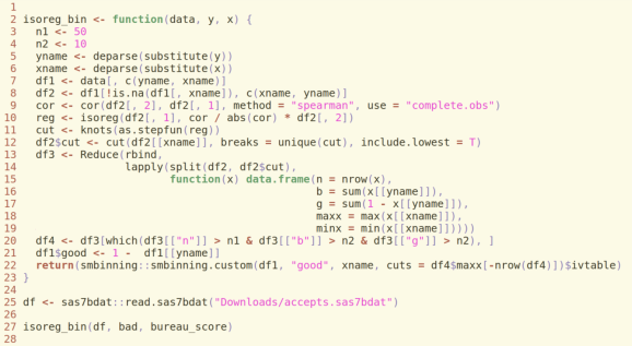
In light of the concern, I revised the function by imposing two thresholds, including a minimum sample size and a minimum number of bads for each bin. Both thresholds can be adjusted based on the specific use case. For instance, I set the minimum sample size equal to 50 and the minimum number of bads (and goods) equal to 10 in the example below. (Since the R code can’t be displayed properly in the wordpress, I have to save it as an image. Please feel free to email me if you want the code.)

As shown in the output, the number of generated bins and the information value happened to be between the result in (https://statcompute.wordpress.com/2017/06/15/finer-monotonic-binning-based-on-isotonic-regression) and the result in (https://statcompute.wordpress.com/2017/01/22/monotonic-binning-with-smbinning-package). More importantly, given a larger sample size for each bin, the binning algorithm is more robust and generalizable.

   Cutpoint CntRec CntGood CntBad CntCumRec CntCumGood CntCumBad PctRec GoodRate BadRate    Odds  LnOdds     WoE     IV
1    <= 559     79      34     45        79         34        45 0.0135   0.4304  0.5696  0.7556 -0.2803 -1.6362 0.0496
2    <= 602    189     102     87       268        136       132 0.0324   0.5397  0.4603  1.1724  0.1591 -1.1969 0.0608
3    <= 605     56      31     25       324        167       157 0.0096   0.5536  0.4464  1.2400  0.2151 -1.1408 0.0162
4    <= 632    468     279    189       792        446       346 0.0802   0.5962  0.4038  1.4762  0.3895 -0.9665 0.0946
5    <= 639    150      95     55       942        541       401 0.0257   0.6333  0.3667  1.7273  0.5465 -0.8094 0.0207
6    <= 653    451     300    151      1393        841       552 0.0773   0.6652  0.3348  1.9868  0.6865 -0.6694 0.0412
7    <= 662    295     213     82      1688       1054       634 0.0505   0.7220  0.2780  2.5976  0.9546 -0.4014 0.0091
8    <= 665    100      77     23      1788       1131       657 0.0171   0.7700  0.2300  3.3478  1.2083 -0.1476 0.0004
9    <= 667     57      44     13      1845       1175       670 0.0098   0.7719  0.2281  3.3846  1.2192 -0.1367 0.0002
10   <= 677    381     300     81      2226       1475       751 0.0653   0.7874  0.2126  3.7037  1.3093 -0.0466 0.0001
11   <= 679     66      53     13      2292       1528       764 0.0113   0.8030  0.1970  4.0769  1.4053  0.0494 0.0000
12   <= 683    160     129     31      2452       1657       795 0.0274   0.8062  0.1938  4.1613  1.4258  0.0699 0.0001
13   <= 689    203     164     39      2655       1821       834 0.0348   0.8079  0.1921  4.2051  1.4363  0.0804 0.0002
14   <= 699    304     249     55      2959       2070       889 0.0521   0.8191  0.1809  4.5273  1.5101  0.1542 0.0012
15   <= 707    312     268     44      3271       2338       933 0.0535   0.8590  0.1410  6.0909  1.8068  0.4509 0.0094
16   <= 717    368     318     50      3639       2656       983 0.0630   0.8641  0.1359  6.3600  1.8500  0.4941 0.0132
17   <= 721    134     119     15      3773       2775       998 0.0230   0.8881  0.1119  7.9333  2.0711  0.7151 0.0094
18   <= 739    474     438     36      4247       3213      1034 0.0812   0.9241  0.0759 12.1667  2.4987  1.1428 0.0735
19   <= 746    166     154     12      4413       3367      1046 0.0284   0.9277  0.0723 12.8333  2.5520  1.1961 0.0277
20      746   1109    1064     45      5522       4431      1091 0.1900   0.9594  0.0406 23.6444  3.1631  1.8072 0.3463
21  Missing    315     210    105      5837       4641      1196 0.0540   0.6667  0.3333  2.0000  0.6931 -0.6628 0.0282
22    Total   5837    4641   1196        NA         NA        NA 1.0000   0.7951  0.2049  3.8804  1.3559  0.0000 0.8021