This post will investigate using Principal Components as part of a momentum strategy.

Recently, I ran across a post from David Varadi that I thought I’d further investigate and translate into code I can explicitly display (as David Varadi doesn’t). Of course, as David Varadi is a quantitative research director with whom I’ve done good work with in the past, I find that trying to investigate his ideas is worth the time spent.

So, here’s the basic idea: in an allegedly balanced universe, containing both aggressive (e.g. equity asset class ETFs) assets and defensive assets (e.g. fixed income asset class ETFs), that principal component analysis, a cornerstone in machine learning, should have some effectiveness at creating an effective portfolio.

I decided to put that idea to the test with the following algorithm:

Using the same assets that David Varadi does, I first use a rolling window (between 6-18 months) to create principal components. Making sure that the SPY half of the loadings is always positive (that is, if the loading for SPY is negative, multiply the first PC by -1, as that’s the PC we use), and then create two portfolios–one that’s comprised of the normalized positive weights of the first PC, and one that’s comprised of the negative half.

Next, every month, I use some momentum lookback period (1, 3, 6, 10, and 12 months), and invest in the portfolio that performed best over that period for the next month, and repeat.

Here’s the source code to do that: (and for those who have difficulty following, I highly recommend James Picerno’s Quantitative Investment Portfolio Analytics in R book.

require(PerformanceAnalytics)
require(quantmod)
require(stats)
require(xts)

symbols <- c("SPY", "EFA", "EEM", "DBC", "HYG", "GLD", "IEF", "TLT")  

# get free data from yahoo
rets <- list()
getSymbols(symbols, src = 'yahoo', from = '1990-12-31')
for(i in 1:length(symbols)) {
  returns <- Return.calculate(Ad(get(symbols[i])))
  colnames(returns) <- symbols[i]
  rets[[i]] <- returns
}
rets <- na.omit(do.call(cbind, rets2))

# 12 month PC rolling PC window, 3 month momentum window
pcPlusMinus <- function(rets, pcWindow = 12, momWindow = 3) {
  ep <- endpoints(rets)

  wtsPc1Plus <- NULL
  wtsPc1Minus <- NULL
  
  for(i in 1:(length(ep)-pcWindow)) {
    # get subset of returns
    returnSubset <- rets[(ep[i]+1):(ep[i+pcWindow])]
    
    # perform PCA, get first PC (I.E. pc1)
    pcs <- prcomp(returnSubset) 
    firstPc <- pcs[[2]][,1]
    
    # make sure SPY always has a positive loading
    # otherwise, SPY and related assets may have negative loadings sometimes
    # positive loadings other times, and creates chaotic return series
    
    if(firstPc['SPY'] < 0) {
      firstPc <- firstPc * -1
    }
    
    # create vector for negative values of pc1
    wtsMinus <- firstPc * -1
    wtsMinus[wtsMinus < 0] <- 0
    wtsMinus <- wtsMinus/(sum(wtsMinus)+1e-16) # in case zero weights
    wtsMinus <- xts(t(wtsMinus), order.by=last(index(returnSubset)))
    wtsPc1Minus[[i]] <- wtsMinus
    
    # create weight vector for positive values of pc1
    wtsPlus <- firstPc
    wtsPlus[wtsPlus < 0] <- 0
    wtsPlus <- wtsPlus/(sum(wtsPlus)+1e-16)
    wtsPlus <- xts(t(wtsPlus), order.by=last(index(returnSubset)))
    wtsPc1Plus[[i]] <- wtsPlus
  }
  
  # combine positive and negative PC1 weights
  wtsPc1Minus <- do.call(rbind, wtsPc1Minus)
  wtsPc1Plus <- do.call(rbind, wtsPc1Plus)
  
  # get return of PC portfolios
  pc1MinusRets <- Return.portfolio(R = rets, weights = wtsPc1Minus)
  pc1PlusRets <- Return.portfolio(R = rets, weights = wtsPc1Plus)
  
  # combine them
  combine <-na.omit(cbind(pc1PlusRets, pc1MinusRets))
  colnames(combine) <- c("PCplus", "PCminus")
  
  momEp <- endpoints(combine)
  momWts <- NULL
  for(i in 1:(length(momEp)-momWindow)){
    momSubset <- combine[(momEp[i]+1):(momEp[i+momWindow])]
    momentums <- Return.cumulative(momSubset)
    momWts[[i]] <- xts(momentums==max(momentums), order.by=last(index(momSubset)))
  }
  momWts <- do.call(rbind, momWts)
  
  out <- Return.portfolio(R = combine, weights = momWts)
  colnames(out) <- paste("PCwin", pcWindow, "MomWin", momWindow, sep="_")
  return(list(out, wtsPc1Minus, wtsPc1Plus, combine))
}


pcWindows <- c(6, 9, 12, 15, 18)
momWindows <- c(1, 3, 6, 10, 12)

permutes <- expand.grid(pcWindows, momWindows)

stratStats <- function(rets) {
  stats <- rbind(table.AnnualizedReturns(rets), maxDrawdown(rets))
  stats[5,] <- stats[1,]/stats[4,]
  stats[6,] <- stats[1,]/UlcerIndex(rets)
  rownames(stats)[4] <- "Worst Drawdown"
  rownames(stats)[5] <- "Calmar Ratio"
  rownames(stats)[6] <- "Ulcer Performance Index"
  return(stats)
}

results <- NULL
for(i in 1:nrow(permutes)) {
  tmp <- pcPlusMinus(rets = rets, pcWindow = permutes$Var1[i], momWindow = permutes$Var2[i])
  results[[i]] <- tmp[[1]]
}
results <- do.call(cbind, results)
stats <- stratStats(results)

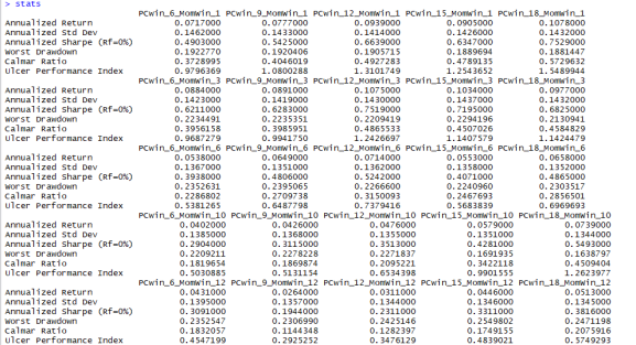
After a cursory look at the results, it seems the performance is fairly miserable with my implementation, even by the standards of tactical asset allocation models (the good ones have a Calmar and Sharpe Ratio above 1)

Here are histograms of the Calmar and Sharpe ratios.

These values are generally too low for my liking. Here’s a screenshot of the table of all 25 results.

While my strategy of choosing which portfolio to hold is different from David Varadi’s (momentum instead of whether or not the aggressive portfolio is above its 200-day moving average), there are numerous studies that show these two methods are closely related, yet the results feel starkly different (and worse) compared to his site.

I’d certainly be willing to entertain suggestions as to how to improve the process, which will hopefully create some more meaningful results. I also know that AllocateSmartly expressed interest in implementing something along these lines for their estimable library of TAA strategies, so I thought I’d try to do it and see what results I’d find, which in this case, aren’t too promising.

Thanks for reading.

NOTE: I am networking, and actively seeking a position related to my skill set in either Philadelphia, New York City, or remotely. If you know of a position which may benefit from my skill set, feel free to let me know. You can reach me on my LinkedIn profile here, or email me.