The 2018 FIFA World Cup has been over for a month now but the memories are far from fading. It was a fabulous tournament, combining underdog stories, upsets, and some pretty high quality football.

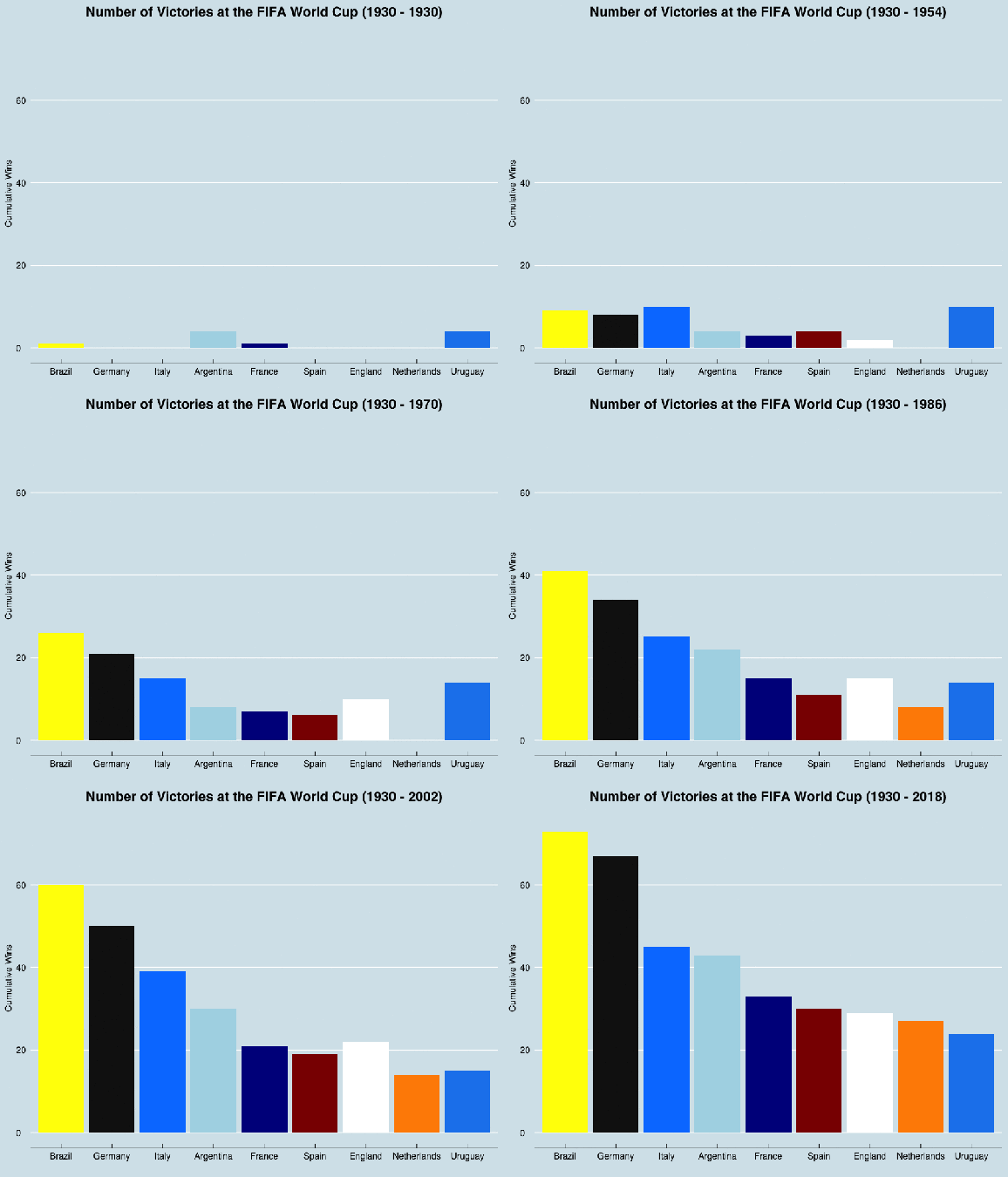
The World Cup has been around for 88 years now, featuring 79 national teams and over 900 matches played. Kaggle’s International Football Results dataset provides a list of all international matches, including every World Cup contest. I decided to count the number of wins from each team and visualize it on an animated bar graph. To make it more readable, I only kept countries that had a cumulative win count of 20+. That left us with nine nations and the following plot:

And here is the R code:

Pre-Processing: Load packages, Load data, Filter to only WC matches, Create “winner” variable, Create “year” variable

library(dplyr)
library(ggplot2)
library(readr)
library(lubridate)
library(animation)
library(ggthemes)

df <- read_csv("results.csv")

world_cup <- df %>% filter(tournament == "FIFA World Cup")

world_cup <- world_cup %>% 
mutate(winner = ifelse(world_cup$home_score > world_cup$away_score, 
world_cup$home_team, 
ifelse(world_cup$away_score > world_cup$home_score,
world_cup$away_team,
"Draw")))

world_cup$year <- world_cup$date %>% year()

Filter to only teams with greater or equal to 20 wins, Complete rows so that every winner has a row for each year, and Create cumulative-wins variable

top_teams <- world_cup %>% filter(winner %in% c( "Brazil",
                                           "Germany",
                                           "Italy",
                                           "Argentina",
                                           "France",
                                           "Spain",
                                           "England",
                                           "Netherlands",
                                           "Uruguay" ))
#complete rows
top_teams <- top_teams %>% 
group_by(year, winner) %>%
count() %>%
ungroup() %>%
complete(year,winner, fill = list(n=0))

#create cumulative sum variable, grouped by winner
top_teams <- top_teams %>%
group_by(winner) %>%
mutate(cs=cumsum(n))

Create gif from GGPLOT

i <- 1930
saveGIF({
for (i in c(1930,1934,1938,1950,1954,1958,1962,1966,1970,1974,1978,
            1982,1986,1990,1994,1998,2002,2006,2010,2014,2018)) {

year_games <- as.character(i)

year_data <- top_teams %>% filter(year == i)

gg <- year_data %>% ggplot(aes(x = winner,
y = cs,
frame = year,
group = winner,
fill = winner)) +
xlim(c("Brazil",
"Germany",
"Italy",
"Argentina",
"France",
"Spain",
"England",
"Netherlands" ,
"Uruguay" )) +
ylim(0,75) +
geom_bar(stat = "identity")+
ggtitle(paste0("Number of Victories at the FIFA World Cup (1930 - ",
                year_games,")")) +
scale_colour_brewer(palette = "Set1") +
labs(x = "", y = "Cumulative Wins")+
theme_dark()+
guides(fill=FALSE) +
theme(panel.grid.major = element_blank(), 
panel.grid.minor = element_blank(),
plot.title = element_text(hjust = 0.5, face = "bold", size = 18),
axis.text.x = element_text(face = "bold", size = 14),
axis.title.y = element_text(face = "bold", size = 14),
axis.text.y = element_text(face = "bold", size = 14)) +
scale_fill_manual(values = c("Brazil" = "yellow1",
"Germany" = "gray8",
"Italy" = "#007FFF",
"Argentina" = "lightblue",
"France" = "darkblue",
"Spain"= "darkred",
"England" = "white",
"Netherlands" = "darkorange",
"Uruguay" = "dodgerblue2")) 



print(gg)

}
}, movie.name = 'world_cup_histogram.gif', interval = 0.8, 
   ani.width = 1500, ani.height = 900)

Code can be found on Github. A big thanks to David Smith at Revolution Analytics, whose blog post helped me a lot in creating the visual.