Hi everyone! In this series we are going to work with a gene called the Mitochondrial Control Region. This series will be about getting some insights into it from sequence analysis. We are going through the entire process, from getting data to reach some conclusions and more importantly raise some questions.

Hugo Bendahan’s Carpincho grazing mitochondrions. Kindly contributed from https://gioiaseyes.wordpress.com/

All of the bash scripts and R functions used in this post are available in our Github, each function is properly linked out to it and we have not uploaded the raw data used in this post for memory reasons and also because this kind of data is ever evolving, nevertheless all the data which is not in our Github is linked out to the respective NCBI server and available for anyone.

Specifically, in this post we are going to do one of the most simple and sometimes most laborious thing to do, getting the data out from the chaotic and well ordered universe of sequences, annotations and variegated ids of databases.

To do this we are going to:

• Download nucleotide sequences (using a web-server)
• Parse large genbank files (.gbff) in R, but using bash scripts.

Since we are going to work with mitochondrial sequences we want to download full mitochondrial genomes (in .gbff format) from the NCBI’s RefSeq ftp server. The reason for using this specific database is that the RefSeq database has two important properties that we are interested in: First, the database is non-redundant and second, it is well annotated. For more of the Refseq’s collection features check their website.

As we know R has some memory issues when dealing with large files, so loading ~600 MB or more as an object in R for further processing is a bit complicated and perhaps it is not the better approach. Because of that we are going to write some Bash scripts to process the data with R but externally to it (using bash and other GNU tools).

The mitochondrial gene that we are interested in is called the ‘Control region’, but for now we are not going to talk about it because the first thing that we need to do is to get the data.

Once we’ve downloaded the data into our local drive we need to parse it. We chose the .gbff file format because it has some other information that we may be interested in. Here arises the first problem when we try to load this large file in R (~614 MB with more than 10 million lines): My computer together with R almost explodes. Well… no, but seriously it gets stuck and runs slow, really slow, so it is really impractical.

So as we can’t just load the data into R to parse it,  we need to devise some kind of plan to work with it. For now, we may ask ourselves the following questions:

1. Of all of the mitochondrial sequences that we have (8866 genomes), in which of them are we really interested in?
2. Are we interested in complete mitochondrial genomes?

In the case of the first question, we are going to define a taxonomic criterion to subset our dataset. We could choose any of the available taxa, but we are going  to restrict our search into one specific suborder of Rodentia: the Hystricomorpha. And the second answer is: Yes we are going to keep the full genomes because we are interested in what happens with other genes of the same macromolecule (mtDNA) and to make comparisons between them and our region of interest.

Therefore  we need to restrict our dataset into every genome that is part of the Hystricomorpha suborder of rodents.

Consequently, what we need then is to progressively subset our dataset into a manageable dataset for R. So, this means that we need to subset the ~600 MB file into a more “discreet one” but sufficiently informative so we can still have the information that we need.

Roughly, the idea is represented in the following figure:

If we check again the structure of a gb/gbf/gbff file then we can see that it has some taxonomic information which is stored in each entry in the following field:

FEATURES → SOURCE → /db_xref=”taxon:

In this field we have a number that it is related to the NCBI taxonomy database (see the disclaimer in the NCBI website if you are a taxonomist!), and with this number, we can know if a particular entry is an hystricomorph or not using another file named nodes.dmp from the taxdmp file located here.

Then, in order to parse this large .gbff file using R we wrote some functions in Bash using the following GNU programs:

• GNU Awk 4.0.1
• GNU bash, version 4.3.11(1)-release (x86_64-pc-linux-gnu)
• cmp (GNU diffutils) 3.3
• grep (GNU grep) 2.16
• sed (GNU sed) 4.2.2

The figure below shows an algorithm which give us an idea in how to do this task.

For each one of these processes (A, B, C and D) we are going to write different bash scripts and R functions. The idea is that every one of these scripts and functions would give us some output files to work in R. Each one of the R functions have some Bash script associated with. Ok, let start.

A – Generating an index of each one of the entries in the .gbff file

In this section we use an R function called CreateCSVFromGBFF() that uses a bash script named CreateCSVFromGBFF.sh. This function takes as input a .gbff file and gives us an output file saved in the working directory as ./csv_files/indexes_summary.csv. For example:

#Run the function to generate a .csv index of the .gbff file
CreateCSVFromGBFF("../raw_data/mitochondrion.1.2.genomic.gbff")
index_mitochondrion <- read.csv(".csv_files/indexes_summary.csv")
str(index_mitochondrion)

'data.frame':	8868 obs. of  8 variables:
 $ fromLine         : Factor w/ 8868 levels "1","10000512",..: 1 416 1437 2347 3196 4184 4998 7369 8236 408 ...
 $ toLine           : int  1043 2091 3140 4077 5133 6090 8454 9378 10392 11405 ...
 $ taxonId          : int  123685 291360 104659 648471 123683 182643 536035 83285 244518 8150 ...
 $ organism         : Factor w/ 8803 levels "","Abacion magnum",..: 5700 5695 5698 358 5696 2067 1359 3939 6142 8460 ...
 $ definition       : Factor w/ 8856 levels ""," 1986"," 1989)",..: 5768 5763 5766 358 5764 2108 1380 3994 6202 8524 ...
 $ locus            : Factor w/ 8867 levels "","AC_000022 16300 bp DNA circular ROD 28-AUG-2012",..: 1855 1856 1858 2267 1860 2305 3872 2888 3078 3079 ...
 $ accession        : Factor w/ 8867 levels "","AC_000022",..: 1853 1854 1856 2266 1858 2304 3872 2888 3078 3079 ...
 $ accession_version: Factor w/ 8867 levels "","AC_000022.2",..: 1853 1854 1856 2266 1858 2304 3872 2888 3078 3079 ...

We can see here that the .csv file has some basic information given in the gbff file and furthermore we add two more columns named fromLine and toLine which have the line number corresponding to the each entry in the .gbff input file. These line numbers along with the taxonId column are the information that we are going to use to further processing the dataset.
Essentially we’ve condensed the information present in the .gbff file into a .csv that can be read as a data.frame in R. We went from a ~600 MB file to a ~1.5 MB file which is a lot better (actually ~400x less memory) to work with.

Now if we go again to the NCBI’s taxonomy browser and look into the Hystricomorpha’s entry we can see that it has a field called “Taxonomy id” (taxid) that is a number, in this case, 33550. This Id is unique to the Hystricomorpha entry and each entry (either a genus, species, subspecies, order, etc.) has a unique one. So now, we need to know which taxids belongs to the Hystricomorpha suborder. And this is part of the following section.

B – Generating a list of child taxids

This part answers to the following question. Given an arbitrary NCBI taxonomic id (parent id): Which are all of the taxids that are below the parent id?. In other words: Which are the child taxids to a given parent taxid?
In order to answer this question more data is required, we need to know the complete list of records of the NCBI’s taxonomy. We have this data at hand (thanks to NCBI) in the taxdmp.zip, more specifically we’ll work with the nodes.dmp file which has the information that we want.

In this particular case we are going to use the bash script: GetNCBITaxonomyChildNodes.sh into the R function called GetNCBITaxonomyChildNodes(). This R function writes a .csv file called ./csv_files/child_nodes.csv that later can be read as a data.frame in R, for example:

# Run the function
GetNCBITaxonomyChildNodes(nodes.dmp.path = "../raw_data/taxdmp/nodes.dmp", target.taxid = "33550")
# Read the .csv output file
child.taxids.df <- read.csv("csv_files/child_nodes.csv", sep="|", header = T)

Afterwards we can make an exploratory plot of the distribution of ranks which are Hystricomorpha’s child nodes.

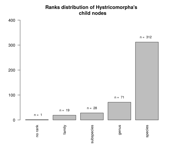
Here we can see that we have 340 taxids in the lower nodes (species + subspecies) and an odd one that has no rank. A search in the taxonomy browser for this taxid returns that is an unclassified Ctenomys, and given that Ctenomys is an hystricomorph then it’s ok.
The next thing that we need to do is to filter our first dataset (output file of the CreateCSVFromGBFF() function of section A) with another function we wrote called FilterParsedGBFF() running the following code:

filtered.gbff.index <- FilterParsedGBFF(path.to.parsed.gbff.csv = "csv_files/indexes_summary.csv", path.to.child.taxids.csv = "csv_files/child_nodes.csv")

Which give us 23 results, this means that we only have 23 complete mitochondrial genomes out of approximately 340 (species+subspecies). This is less than 7% of all hystricomorphs mitochondrial genomes are actually sequenced.

In conclusion:

1. We have got all the child taxids of a given parent taxid in the NCBI’s taxonomy database.
2. We have subsetted a larger database by using the taxonomic units of interest (from 8866 entries to 23).

C and D – Extracting individual .gbff and .fasta sequence files

Now with the last filtered database we can finally extract from the large ~600 MB file the individual .gbff and .fasta entries.

ExtractFilteredGBFFFromCSV(path.to.filtered.CSV = "csv_files/filtered.csv",path.to.gbff.sourcefile = "../raw_data/mitochondrion.1.2.genomic.gbff")
ExtractFastaSeqsFromGBFF(path.to.folder.with.gbff.files = "gbff_filtered_files/")

The ExtractFilteredGBFFFromCSV() uses the filtered.csv file which have the line number of each entry within the source .gbff file, and it returns individual .gbff files (23 in this case) in the directory ./gbff_filtered_files/ named according to the following format: Organism Name + Accession number like for example: Ctenomys_sociabilis_NC_020658.gbff
After extracting each entry to separate .gbff files we use ExtractFastaSeqsFromGBFF() in the following way:

# Run the function
ExtractFastaSeqsFromGBFF(path.to.folder.with.gbff.files = "gbff_filtered_files/")

And finally all the .fasta files will be saved into the folder ./gbff_filtered_files/fasta_seqs/.

The last two R functions also use the corresponding bash scripts:

• ExtractFilteredGBFFFromCSV.sh
• ExtractFastaSeqsFromGBFF.sh

Conclusion, limitations and final remarks

• We have successfully filtered a large .gbff file using R + Bash overcoming the memory limitations when loading large datasets in R. Bypassing this with Bash creating local files instead of loading every middle step of the workflow into the memory in R
• There could be some compatibility issues when trying to use the bash scripts in other operating systems rather than Linux. If it’s necessary this could be worked out.

The figure below gives us a final understanding of this post’s workflow, the different scripts+functions used, and also the files and temporary folders created.