
Practical Machine Learning with R and Python – Part 1
Want to share your content on R-bloggers? click here if you have a blog, or here if you don't.
Introduction
This is the 1st part of a series of posts I intend to write on some common Machine Learning Algorithms in R and Python. In this first part I cover the following Machine Learning Algorithms
- Univariate Regression
- Multivariate Regression
- Polynomial Regression
- K Nearest Neighbors Regression
The code includes the implementation in both R and Python. This series of posts are based on the following 2 MOOC courses I did at Stanford Online and at Coursera
- Statistical Learning, Prof Trevor Hastie & Prof Robert Tibesherani, Online Stanford
- Applied Machine Learning in Python Prof Kevyn-Collin Thomson, University Of Michigan, Coursera
I have used the data sets from UCI Machine Learning repository(Communities and Crime and Auto MPG). I also use the Boston data set from MASS package
While coding in R and Python I found that there were some aspects that were more convenient in one language and some in the other. For example, plotting the fit in R is straightforward in R, while computing the R squared, splitting as Train & Test sets etc. are already available in Python. In any case, these minor inconveniences can be easily be implemented in either language.
R squared computation in R is computed as follows
^{2}")
)^{2}")

Note: You can download this R Markdown file and the associated data sets from Github at MachineLearning-RandPython
Note 1: This post was created as an R Markdown file in RStudio which has a cool feature of including R and Python snippets. The plot of matplotlib needs a workaround but otherwise this is a real cool feature of RStudio!
1.1a Univariate Regression – R code
Here a simple linear regression line is fitted between a single input feature and the target variable
# Source in the R function library
source("RFunctions.R")
# Read the Boston data file
df=read.csv("Boston.csv",stringsAsFactors = FALSE) # Data from MASS - Statistical Learning

# Split the data into training and test sets (75:25)
train_idx <- trainTestSplit(df,trainPercent=75,seed=5)
train <- df[train_idx, ]
test <- df[-train_idx, ]

# Fit a linear regression line between 'Median value of owner occupied homes' vs 'lower status of
# population'
fit=lm(medv~lstat,data=df)
# Display details of fir
summary(fit)
##
## Call:
## lm(formula = medv ~ lstat, data = df)
##
## Residuals:
##     Min      1Q  Median      3Q     Max
## -15.168  -3.990  -1.318   2.034  24.500
##
## Coefficients:
##             Estimate Std. Error t value Pr(>|t|)
## (Intercept) 34.55384    0.56263   61.41   <2e-16 ***
## lstat       -0.95005    0.03873  -24.53   <2e-16 ***
## ---
## Signif. codes:  0 '***' 0.001 '**' 0.01 '*' 0.05 '.' 0.1 ' ' 1
##
## Residual standard error: 6.216 on 504 degrees of freedom
## Multiple R-squared:  0.5441, Adjusted R-squared:  0.5432
## F-statistic: 601.6 on 1 and 504 DF,  p-value: < 2.2e-16
# Display the confidence intervals
confint(fit)
##                 2.5 %     97.5 %
## (Intercept) 33.448457 35.6592247
## lstat       -1.026148 -0.8739505
plot(df$lstat,df$medv, xlab="Lower status (%)",ylab="Median value of owned homes ($1000)", main="Median value of homes ($1000) vs Lowe status (%)")
abline(fit)
abline(fit,lwd=3)
abline(fit,lwd=3,col="red")

rsquared=Rsquared(fit,test,test$medv)
sprintf("R-squared for uni-variate regression (Boston.csv)  is : %f", rsquared)
## [1] "R-squared for uni-variate regression (Boston.csv)  is : 0.556964"
1.1b Univariate Regression – Python code
import numpy as np
import pandas as pd
import os
import matplotlib.pyplot as plt
from sklearn.model_selection import train_test_split
from sklearn.linear_model import LinearRegression
#os.chdir("C:\\software\\machine-learning\\RandPython")

# Read the CSV file
df = pd.read_csv("Boston.csv",encoding = "ISO-8859-1")
# Select the feature variable
X=df['lstat']

# Select the target
y=df['medv']

# Split into train and test sets (75:25)
X_train, X_test, y_train, y_test = train_test_split(X, y,random_state = 0)
X_train=X_train.values.reshape(-1,1)
X_test=X_test.values.reshape(-1,1)

# Fit a linear model
linreg = LinearRegression().fit(X_train, y_train)

# Print the training and test R squared score
print('R-squared score (training): {:.3f}'.format(linreg.score(X_train, y_train)))
print('R-squared score (test): {:.3f}'.format(linreg.score(X_test, y_test)))

# Plot the linear regression line
fig=plt.scatter(X_train,y_train)

# Create a range of points. Compute yhat=coeff1*x + intercept and plot
x=np.linspace(0,40,20)
fig1=plt.plot(x, linreg.coef_ * x + linreg.intercept_, color='red')
fig1=plt.title("Median value of homes ($1000) vs Lowe status (%)")
fig1=plt.xlabel("Lower status (%)")
fig1=plt.ylabel("Median value of owned homes ($1000)")
fig.figure.savefig('foo.png', bbox_inches='tight')
fig1.figure.savefig('foo1.png', bbox_inches='tight')
print "Finished"

## R-squared score (training): 0.571
## R-squared score (test): 0.458
## Finished

1.2a Multivariate Regression – R code
# Read crimes data
crimesDF <- read.csv("crimes.csv",stringsAsFactors = FALSE)

# Remove the 1st 7 columns which do not impact output
crimesDF1 <- crimesDF[,7:length(crimesDF)]

# Convert all to numeric
crimesDF2 <- sapply(crimesDF1,as.numeric)

# Check for NAs
a <- is.na(crimesDF2)
# Set to 0 as an imputation
crimesDF2[a] <-0
#Create as a dataframe
crimesDF2 <- as.data.frame(crimesDF2)
#Create a train/test split
train_idx <- trainTestSplit(crimesDF2,trainPercent=75,seed=5)
train <- crimesDF2[train_idx, ]
test <- crimesDF2[-train_idx, ]

# Fit a multivariate regression model between crimesPerPop and all other features
fit <- lm(ViolentCrimesPerPop~.,data=train)

# Compute and print R Squared
rsquared=Rsquared(fit,test,test$ViolentCrimesPerPop)
sprintf("R-squared for multi-variate regression (crimes.csv)  is : %f", rsquared)
## [1] "R-squared for multi-variate regression (crimes.csv)  is : 0.653940"
1.2b Multivariate Regression – Python code
import numpy as np
import pandas as pd
import os
import matplotlib.pyplot as plt
from sklearn.model_selection import train_test_split
from sklearn.linear_model import LinearRegression
# Read the data
crimesDF =pd.read_csv("crimes.csv",encoding="ISO-8859-1")
#Remove the 1st 7 columns
crimesDF1=crimesDF.iloc[:,7:crimesDF.shape[1]]
# Convert to numeric
crimesDF2 = crimesDF1.apply(pd.to_numeric, errors='coerce')
# Impute NA to 0s
crimesDF2.fillna(0, inplace=True)

# Select the X (feature vatiables - all)
X=crimesDF2.iloc[:,0:120]

# Set the target
y=crimesDF2.iloc[:,121]

X_train, X_test, y_train, y_test = train_test_split(X, y,random_state = 0)
# Fit a multivariate regression model
linreg = LinearRegression().fit(X_train, y_train)

# compute and print the R Square
print('R-squared score (training): {:.3f}'.format(linreg.score(X_train, y_train)))
print('R-squared score (test): {:.3f}'.format(linreg.score(X_test, y_test)))
## R-squared score (training): 0.699
## R-squared score (test): 0.677
1.3a Polynomial Regression – R
For Polynomial regression , polynomials of degree 1,2 & 3 are used and R squared is computed. It can be seen that the quadaratic model provides the best R squared score and hence the best fit
 # Polynomial degree 1
df=read.csv("auto_mpg.csv",stringsAsFactors = FALSE) # Data from UCI
df1 <- as.data.frame(sapply(df,as.numeric))

# Select key columns
df2 <- df1 %>% select(cylinder,displacement, horsepower,weight, acceleration, year,mpg)
df3 <- df2[complete.cases(df2),]

# Split as train and test sets
train_idx <- trainTestSplit(df3,trainPercent=75,seed=5)
train <- df3[train_idx, ]
test <- df3[-train_idx, ]

# Fit a model of degree 1
fit <- lm(mpg~. ,data=train)
rsquared1 <-Rsquared(fit,test,test$mpg)
sprintf("R-squared for Polynomial regression of degree 1 (auto_mpg.csv)  is : %f", rsquared1)
## [1] "R-squared for Polynomial regression of degree 1 (auto_mpg.csv)  is : 0.763607"
# Polynomial degree 2 - Quadratic
x = as.matrix(df3[1:6])
# Make a  polynomial  of degree 2 for feature variables before split
df4=as.data.frame(poly(x,2,raw=TRUE))
df5 <- cbind(df4,df3[7])

# Split into train and test set
train_idx <- trainTestSplit(df5,trainPercent=75,seed=5)
train <- df5[train_idx, ]
test <- df5[-train_idx, ]

# Fit the quadratic model
fit <- lm(mpg~. ,data=train)
# Compute R squared
rsquared2=Rsquared(fit,test,test$mpg)
sprintf("R-squared for Polynomial regression of degree 2 (auto_mpg.csv)  is : %f", rsquared2)
## [1] "R-squared for Polynomial regression of degree 2 (auto_mpg.csv)  is : 0.831372"
#Polynomial degree 3
x = as.matrix(df3[1:6])
# Make polynomial of degree 4  of feature variables before split
df4=as.data.frame(poly(x,3,raw=TRUE))
df5 <- cbind(df4,df3[7])
train_idx <- trainTestSplit(df5,trainPercent=75,seed=5)

train <- df5[train_idx, ]
test <- df5[-train_idx, ]
# Fit a model of degree 3
fit <- lm(mpg~. ,data=train)
# Compute R squared
rsquared3=Rsquared(fit,test,test$mpg)
sprintf("R-squared for Polynomial regression of degree 2 (auto_mpg.csv)  is : %f", rsquared3)
## [1] "R-squared for Polynomial regression of degree 2 (auto_mpg.csv)  is : 0.773225"
df=data.frame(degree=c(1,2,3),Rsquared=c(rsquared1,rsquared2,rsquared3))
# Make a plot of Rsquared and degree
ggplot(df,aes(x=degree,y=Rsquared)) +geom_point() + geom_line(color="blue") +
    ggtitle("Polynomial regression - R squared vs Degree of polynomial") +
    xlab("Degree") + ylab("R squared")

1.3a Polynomial Regression – Python
For Polynomial regression , polynomials of degree 1,2 & 3 are used and R squared is computed. It can be seen that the quadaratic model provides the best R squared score and hence the best fit
import numpy as np
import pandas as pd
import os
import matplotlib.pyplot as plt
from sklearn.model_selection import train_test_split
from sklearn.linear_model import LinearRegression
from sklearn.preprocessing import PolynomialFeatures
autoDF =pd.read_csv("auto_mpg.csv",encoding="ISO-8859-1")
autoDF.shape
autoDF.columns
# Select key columns
autoDF1=autoDF[['mpg','cylinder','displacement','horsepower','weight','acceleration','year']]
# Convert columns to numeric
autoDF2 = autoDF1.apply(pd.to_numeric, errors='coerce')
# Drop NAs
autoDF3=autoDF2.dropna()
autoDF3.shape
X=autoDF3[['cylinder','displacement','horsepower','weight','acceleration','year']]
y=autoDF3['mpg']

# Polynomial degree 1
X_train, X_test, y_train, y_test = train_test_split(X, y,random_state = 0)
linreg = LinearRegression().fit(X_train, y_train)
print('R-squared score - Polynomial degree 1 (training): {:.3f}'.format(linreg.score(X_train, y_train)))
# Compute R squared
rsquared1 =linreg.score(X_test, y_test)
print('R-squared score - Polynomial degree 1 (test): {:.3f}'.format(linreg.score(X_test, y_test)))

# Polynomial degree 2
poly = PolynomialFeatures(degree=2)
X_poly = poly.fit_transform(X)
X_train, X_test, y_train, y_test = train_test_split(X_poly, y,random_state = 0)
linreg = LinearRegression().fit(X_train, y_train)

# Compute R squared
print('R-squared score - Polynomial degree 2 (training): {:.3f}'.format(linreg.score(X_train, y_train)))
rsquared2 =linreg.score(X_test, y_test)
print('R-squared score - Polynomial degree 2 (test): {:.3f}\n'.format(linreg.score(X_test, y_test)))

#Polynomial degree 3

poly = PolynomialFeatures(degree=3)
X_poly = poly.fit_transform(X)
X_train, X_test, y_train, y_test = train_test_split(X_poly, y,random_state = 0)
linreg = LinearRegression().fit(X_train, y_train)
print('(R-squared score -Polynomial degree 3  (training): {:.3f}'
     .format(linreg.score(X_train, y_train)))
# Compute R squared
rsquared3 =linreg.score(X_test, y_test)
print('R-squared score Polynomial degree 3 (test): {:.3f}\n'.format(linreg.score(X_test, y_test)))
degree=[1,2,3]
rsquared =[rsquared1,rsquared2,rsquared3]
fig2=plt.plot(degree,rsquared)
fig2=plt.title("Polynomial regression - R squared vs Degree of polynomial")
fig2=plt.xlabel("Degree")
fig2=plt.ylabel("R squared")
fig2.figure.savefig('foo2.png', bbox_inches='tight')
print "Finished plotting and saving"

## R-squared score - Polynomial degree 1 (training): 0.811
## R-squared score - Polynomial degree 1 (test): 0.799
## R-squared score - Polynomial degree 2 (training): 0.861
## R-squared score - Polynomial degree 2 (test): 0.847
##
## (R-squared score -Polynomial degree 3  (training): 0.933
## R-squared score Polynomial degree 3 (test): 0.710
##
## Finished plotting and saving

1.4 K Nearest Neighbors
The code below implements KNN Regression both for R and Python. This is done for different neighbors. The R squared is computed in each case. This is repeated after performing feature scaling. It can be seen the model fit is much better after feature scaling. Normalization refers to
}{max(X-min(X))}")
Another technique that is used is Standardization which is
}{sd(X)}")
1.4a K Nearest Neighbors Regression – R( Unnormalized)
The R code below does not use feature scaling
# KNN regression requires the FNN package
df=read.csv("auto_mpg.csv",stringsAsFactors = FALSE) # Data from UCI
df1 <- as.data.frame(sapply(df,as.numeric))
df2 <- df1 %>% select(cylinder,displacement, horsepower,weight, acceleration, year,mpg)
df3 <- df2[complete.cases(df2),]

# Split train and test
train_idx <- trainTestSplit(df3,trainPercent=75,seed=5)
train <- df3[train_idx, ]
test <- df3[-train_idx, ]
#  Select the feature variables
train.X=train[,1:6]
# Set the target for training
train.Y=train[,7]
# Do the same for test set
test.X=test[,1:6]
test.Y=test[,7]

rsquared <- NULL
# Create a list of neighbors
neighbors <-c(1,2,4,8,10,14)
for(i in seq_along(neighbors)){
    # Perform a KNN regression fit
    knn=knn.reg(train.X,test.X,train.Y,k=neighbors[i])
    # Compute R sqaured
    rsquared[i]=knnRSquared(knn$pred,test.Y)
}

# Make a dataframe for plotting
df <- data.frame(neighbors,Rsquared=rsquared)
# Plot the number of neighors vs the R squared
ggplot(df,aes(x=neighbors,y=Rsquared)) + geom_point() +geom_line(color="blue") +
    xlab("Number of neighbors") + ylab("R squared") +
    ggtitle("KNN regression - R squared vs Number of Neighors (Unnormalized)")

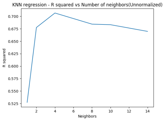
1.4b K Nearest Neighbors Regression – Python( Unnormalized)
The Python code below does not use feature scaling
import numpy as np
import pandas as pd
import os
import matplotlib.pyplot as plt
from sklearn.model_selection import train_test_split
from sklearn.linear_model import LinearRegression
from sklearn.preprocessing import PolynomialFeatures
from sklearn.neighbors import KNeighborsRegressor
autoDF =pd.read_csv("auto_mpg.csv",encoding="ISO-8859-1")
autoDF.shape
autoDF.columns
autoDF1=autoDF[['mpg','cylinder','displacement','horsepower','weight','acceleration','year']]
autoDF2 = autoDF1.apply(pd.to_numeric, errors='coerce')
autoDF3=autoDF2.dropna()
autoDF3.shape
X=autoDF3[['cylinder','displacement','horsepower','weight','acceleration','year']]
y=autoDF3['mpg']

# Perform a train/test split
X_train, X_test, y_train, y_test = train_test_split(X, y, random_state = 0)
# Create a list of neighbors
rsquared=[]
neighbors=[1,2,4,8,10,14]
for i in neighbors:
        # Fit a KNN model
        knnreg = KNeighborsRegressor(n_neighbors = i).fit(X_train, y_train)
        # Compute R squared
        rsquared.append(knnreg.score(X_test, y_test))
        print('R-squared test score: {:.3f}'
        .format(knnreg.score(X_test, y_test)))
# Plot the number of neighors vs the R squared
fig3=plt.plot(neighbors,rsquared)
fig3=plt.title("KNN regression - R squared vs Number of neighbors(Unnormalized)")
fig3=plt.xlabel("Neighbors")
fig3=plt.ylabel("R squared")
fig3.figure.savefig('foo3.png', bbox_inches='tight')
print "Finished plotting and saving"
## R-squared test score: 0.527
## R-squared test score: 0.678
## R-squared test score: 0.707
## R-squared test score: 0.684
## R-squared test score: 0.683
## R-squared test score: 0.670
## Finished plotting and saving
1.4c K Nearest Neighbors Regression – R( Normalized)
It can be seen that R squared improves when the features are normalized.
df=read.csv("auto_mpg.csv",stringsAsFactors = FALSE) # Data from UCI
df1 <- as.data.frame(sapply(df,as.numeric))
df2 <- df1 %>% select(cylinder,displacement, horsepower,weight, acceleration, year,mpg)
df3 <- df2[complete.cases(df2),]

# Perform MinMaxScaling of feature variables
train.X.scaled=MinMaxScaler(train.X)
test.X.scaled=MinMaxScaler(test.X)

# Create a list of neighbors
rsquared <- NULL
neighbors <-c(1,2,4,6,8,10,12,15,20,25,30)
for(i in seq_along(neighbors)){
    # Fit a KNN model
    knn=knn.reg(train.X.scaled,test.X.scaled,train.Y,k=i)
    # Compute R ssquared
    rsquared[i]=knnRSquared(knn$pred,test.Y)

}

df <- data.frame(neighbors,Rsquared=rsquared)
# Plot the number of neighors vs the R squared
ggplot(df,aes(x=neighbors,y=Rsquared)) + geom_point() +geom_line(color="blue") +
    xlab("Number of neighbors") + ylab("R squared") +
    ggtitle("KNN regression - R squared vs Number of Neighors(Normalized)")

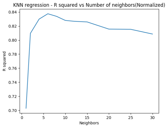
1.4d K Nearest Neighbors Regression – Python( Normalized)
R squared improves when the features are normalized with MinMaxScaling
import numpy as np
import pandas as pd
import os
import matplotlib.pyplot as plt
from sklearn.model_selection import train_test_split
from sklearn.linear_model import LinearRegression
from sklearn.preprocessing import PolynomialFeatures
from sklearn.neighbors import KNeighborsRegressor
from sklearn.preprocessing import MinMaxScaler
autoDF =pd.read_csv("auto_mpg.csv",encoding="ISO-8859-1")
autoDF.shape
autoDF.columns
autoDF1=autoDF[['mpg','cylinder','displacement','horsepower','weight','acceleration','year']]
autoDF2 = autoDF1.apply(pd.to_numeric, errors='coerce')
autoDF3=autoDF2.dropna()
autoDF3.shape
X=autoDF3[['cylinder','displacement','horsepower','weight','acceleration','year']]
y=autoDF3['mpg']

# Perform a train/ test  split
X_train, X_test, y_train, y_test = train_test_split(X, y, random_state = 0)
# Use MinMaxScaling
scaler = MinMaxScaler()
X_train_scaled = scaler.fit_transform(X_train)
# Apply scaling on test set
X_test_scaled = scaler.transform(X_test)

# Create a list of neighbors
rsquared=[]
neighbors=[1,2,4,6,8,10,12,15,20,25,30]
for i in neighbors:
    # Fit a KNN model
    knnreg = KNeighborsRegressor(n_neighbors = i).fit(X_train_scaled, y_train)
    # Compute R squared
    rsquared.append(knnreg.score(X_test_scaled, y_test))
    print('R-squared test score: {:.3f}'
        .format(knnreg.score(X_test_scaled, y_test)))

# Plot the number of neighors vs the R squared
fig4=plt.plot(neighbors,rsquared)
fig4=plt.title("KNN regression - R squared vs Number of neighbors(Normalized)")
fig4=plt.xlabel("Neighbors")
fig4=plt.ylabel("R squared")
fig4.figure.savefig('foo4.png', bbox_inches='tight')
print "Finished plotting and saving"
## R-squared test score: 0.703
## R-squared test score: 0.810
## R-squared test score: 0.830
## R-squared test score: 0.838
## R-squared test score: 0.834
## R-squared test score: 0.828
## R-squared test score: 0.827
## R-squared test score: 0.826
## R-squared test score: 0.816
## R-squared test score: 0.815
## R-squared test score: 0.809
## Finished plotting and saving
Conclusion
In this initial post I cover the regression models when the output is continous. I intend to touch upon other Machine Learning algorithms.
Comments, suggestions and corrections are welcome.
Watch this this space!
To be continued….
You may like
1. Using Linear Programming (LP) for optimizing bowling change or batting lineup in T20 cricket
2. Neural Networks: The mechanics of backpropagation
3. More book, more cricket! 2nd edition of my books now on Amazon
4. Spicing up a IBM Bluemix cloud app with MongoDB and NodeExpress
5. Introducing cricket package yorkr:Part 4-In the block hole!
To see all posts see Index of posts

R-bloggers.com offers daily e-mail updates about R news and tutorials about learning R and many other topics. Click here if you're looking to post or find an R/data-science job.
Want to share your content on R-bloggers? click here if you have a blog, or here if you don't.