The first part of this post is a quick update on Tony Cooper’s of Double Digit Numerics’s volatility ETN momentum strategy from the volatility made simple blog (which has stopped updating as of a year and a half ago). The second part will cover Dr. Jonathan Kinlay’s Beta Convexity concept.

So, now that I have the ability to generate a term structure and constant expiry contracts, I decided to revisit some of the strategies on Volatility Made Simple and see if any of them are any good (long story short: all of the publicly detailed ones aren’t so hot besides mine–they either have a massive drawdown in-sample around the time of the crisis, or a massive drawdown out-of-sample).

Why this strategy? Because it seemed different from most of the usual term structure ratio trades (of which mine is an example), so I thought I’d check out how it did since its first publishing date, and because it’s rather easy to understand.

Here’s the strategy:

Take XIV, VXX, ZIV, VXZ, and SHY (this last one as the “risk free” asset), and at the close, invest in whichever has had the highest 83 day momentum (this was the result of optimization done on volatilityMadeSimple).

Here’s the code to do this in R, using the Quandl EOD database. There are two variants tested–observe the close, buy the close (AKA magical thinking), and observe the close, buy tomorrow’s close.

require(quantmod)
require(PerformanceAnalytics)
require(TTR)
require(Quandl)

Quandl.api_key("yourKeyHere")

symbols <- c("XIV", "VXX", "ZIV", "VXZ", "SHY")

prices <- list()
for(i in 1:length(symbols)) {
  price <- Quandl(paste0("EOD/", symbols[i]), start_date="1990-12-31", type = "xts")$Adj_Close
  colnames(price) <- symbols[i]
  prices[[i]] <- price
}
prices <- na.omit(do.call(cbind, prices))
returns <- na.omit(Return.calculate(prices))

# find highest asset, assign column names
topAsset <- function(row, assetNames) {
  out <- row==max(row, na.rm = TRUE)
  names(out) <- assetNames
  out <- data.frame(out)
  return(out)
}

# compute momentum
momentums <- na.omit(xts(apply(prices, 2, ROC, n = 83), order.by=index(prices)))

# find highest asset each day, turn it into an xts
highestMom <- apply(momentums, 1, topAsset, assetNames = colnames(momentums))
highestMom <- xts(t(do.call(cbind, highestMom)), order.by=index(momentums))

# observe today's close, buy tomorrow's close
buyTomorrow <- na.omit(xts(rowSums(returns * lag(highestMom, 2)), order.by=index(highestMom)))

# observe today's close, buy today's close (aka magic thinking)
magicThinking <- na.omit(xts(rowSums(returns * lag(highestMom)), order.by=index(highestMom)))

out <- na.omit(cbind(buyTomorrow, magicThinking))
colnames(out) <- c("buyTomorrow", "magicalThinking")

# results
charts.PerformanceSummary(out['2014-04-11::'], legend.loc = 'top')
rbind(table.AnnualizedReturns(out['2014-04-11::']), maxDrawdown(out['2014-04-11::']))

Pretty simple.

Here are the results.

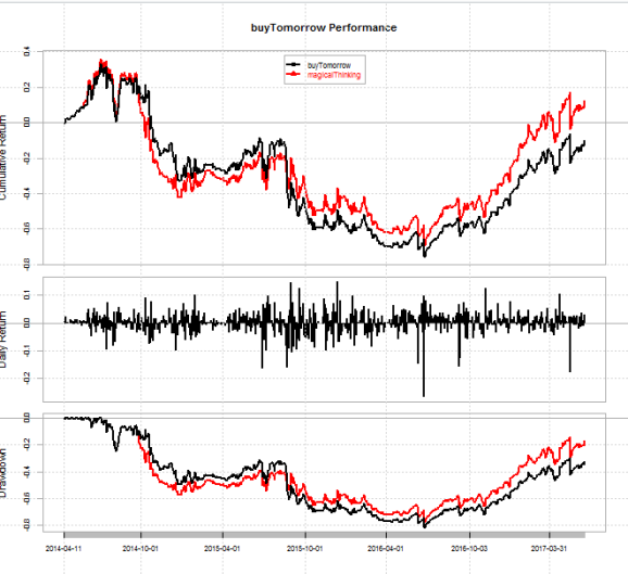
> rbind(table.AnnualizedReturns(out['2014-04-11::']), maxDrawdown(out['2014-04-11::']))
                          buyTomorrow magicalThinking
Annualized Return          -0.0320000       0.0378000
Annualized Std Dev          0.5853000       0.5854000
Annualized Sharpe (Rf=0%)  -0.0547000       0.0646000
Worst Drawdown              0.8166912       0.7761655

Looks like this strategy didn’t pan out too well. Just a daily reminder that if you’re using fine grid-search to select a particularly good parameter (EG n = 83 days? Maybe 4 21-day trading months, but even that would have been n = 82), you’re asking for a visit from, in the words of Mr. Tony Cooper, a visit from the grim reaper.

****

Moving onto another topic, whenever Dr. Jonathan Kinlay posts something that I think I can replicate that I’d be very wise to do so, as he is a very skilled and experienced practitioner (and also includes me on his blogroll).

A topic that Dr. Kinlay covered is the idea of beta convexity–namely, that an asset’s beta to a benchmark may be different when the benchmark is up as compared to when it’s down. Essentially, it’s the idea that we want to weed out firms that are what I’d deem as “losers in disguise”–I.E. those that act fine when times are good (which is when we really don’t care about diversification, since everything is going up anyway), but do nothing during bad times.

The beta convexity is calculated quite simply: it’s the beta of an asset to a benchmark when the benchmark has a positive return, minus the beta of an asset to a benchmark when the benchmark has a negative return, then squaring the difference. That is, (beta_bench_positive – beta_bench_negative) ^ 2.

Here’s some R code to demonstrate this, using IBM vs. the S&P 500 since 1995.

ibm <- Quandl("EOD/IBM", start_date="1995-01-01", type = "xts")
ibmRets <- Return.calculate(ibm$Adj_Close)

spy <- Quandl("EOD/SPY", start_date="1995-01-01", type = "xts")
spyRets <- Return.calculate(spy$Adj_Close)

rets <- na.omit(cbind(ibmRets, spyRets))
colnames(rets) <- c("IBM", "SPY")

betaConvexity <- function(Ra, Rb) {
  positiveBench <- Rb[Rb > 0]
  assetPositiveBench <- Ra[index(positiveBench)]
  positiveBeta <- CAPM.beta(Ra = assetPositiveBench, Rb = positiveBench)
  
  negativeBench <- Rb[Rb < 0]
  assetNegativeBench <- Ra[index(negativeBench)]
  negativeBeta <- CAPM.beta(Ra = assetNegativeBench, Rb = negativeBench)
  
  out <- (positiveBeta - negativeBeta) ^ 2
  return(out)
}

betaConvexity(rets$IBM, rets$SPY)

For the result:

> betaConvexity(rets$IBM, rets$SPY)
[1] 0.004136034

Thanks for reading.

NOTE: I am always looking to network, and am currently actively looking for full-time opportunities which may benefit from my skill set. If you have a position which may benefit from my skills, do not hesitate to reach out to me. My LinkedIn profile can be found here.