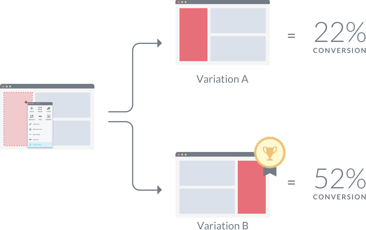
In the field of webpage optimization, A/B testing is the most commonly and widely used experimentation method to compare two (or more) versions of a webpage or app to determine which version performs better in measures like traffic or customer conversion rates. The basic design is to randomly assign your incoming website traffic to one of your website versions with equal probability, collect data, and perform a two proportion test to determine whether performance between versions are statistically significantly different.

However, A/B tests are not ideal in practical applications as they fail to take into consideration the losses incurred during the test. Nowadays a popular alternative to A/B testing known as Multi Armed Bandit experiments are getting a lot of attention. The Multi Armed Bandit model is a form of reinforcement learning that is designed to maximize the gain or minimize the loss during the experiment while collecting sufficient data for hypothesis testing. Here I give an overview of the algorithm behind these experiment designs, discuss its benefits and shortcomings, and simulate the tests to assess the performance of different methods.

Overview

Figure: A/B Test

During an A/B test experiment, an equal portion of samples is assigned to each version, thus the data collected is balanced. Theoretically speaking, this is the best way to collect data and perform hypothesis testing, if the ultimate goal is to find the ground truth on which version is the best. We will call this the “learning” phase (otherwise known as the “exploration” phase).

After some given period of time or number of samples collected, a hypothesis test is performed, at which point all future samples are then assigned to the top performing version. We will call this the “earning” phase (otherwise known as the “exploitation phase”).

Figure: A/B Test Phases

However where A/B test falls short is the ability to maximize the gain or minimize the cost of the experiment. In practice, deliberately assigning samples to a lower performing version may be very costly; for example in clinical trials where an experiment is performed to determine whether or not a drug is effective, if half of the samples are assigned to a placebo drug, those patients receiving a placebo drug may be subject to missing out on a treatment that may be life-saving. In business, assigning samples to a lower performing website may mean the company is missing out on business opportunities.

This is where a Multi Armed Bandit test may be more optimal: a Multi Armed Bandit is designed to maximize gain/minimize loss during the experiment, while simultaneously collecting data to perform hypothesis testing.

A Multi Armed Bandit experiment is designed with a mix of the two phases. During the exploration phase (which is typically shorter in a Multi Armed Bandit test than in an A/B test), samples are randomly and evenly assigned to a version, similar to an A/B test. However after some initial learning phase, samples are assigned proportionally larger to a higher performing version, either immediately or gradually, moving towards the earning phase rather quickly and efficiently.

Figure: Multi Armed Bandit Phases

Methods

Here we introduce some of the popular Multi Armed Bandit algorithms.

Epsilon-Greedy Multi Armed Bandit Test

During the “learning” phase of the Epsilon Greedy Multi Armed Bandit algorithm, the allocation of new samples are determined by a parameter (epsilon), a value between 0 and 1. At any given point during the experiment, the version that has the best performance so far (i.e. has the best proportion of successes to number of trials) is the Best Arm, and during the next round a proportion (1 – epsilon) of all samples are allocated to the best arm. All other samples of proportion (epsilon) are allocated evenly to all other versions (in a two version scenario, (epsilon) samples are allocated to the worse-performing version).

In the binomial trial scenario, the performance of the version is defined as the sum of all successes divided by the number of samples collected for the particular version.

Figure: Epsilon Greedy Multi Armed Bandit

Thus at any given time during the experiment, samples are allocated to all existing versions in the test, but are allocated favorably to the best arm with a proportion (1-epsilon). This way the Best arm is being exploited for its high performance, while collecting samples for other versions simulatenously.

Epsilon-Decreasing Multi Armed Bandit Test

The Epsilon Decreasing Multi Armed Bandit test have a very similar design to the Epsilon Greedy design, with the exception of the epsilon value. In the Epsilon Greedy method, epsilon is a constant across the entire experiment. However in the Epsilon Decreasing design, as the name would suggest, epsilon decreases throughout the experiment by function defined a priori.

Thus similarly to the Epsilon Greedy method, at any given time during the experiment, samples are collected for versions, but favorably to the best arm at an increasing rate of the proportion 1 – epsilon.

UCB1 Multi Armed Bandit Test

The Upper Confidence Bound (UCB1) Multi Armed Bandit algorithm is a more intricate algorithm that considers the uncertainty of determining the best arm at any given time in the experiment, or otherwise known to be robust in the “Optimism in the face of uncertainty”

Unlike the Epsilon methods, after the learning phase all samples are allocated to the best arm only. The UCB1 design distinguishes itself from the other methods in determining the best arm. Unlike the previous two methods where the best arm is determined by the actual performance of the versions, in the UCB1 algorithm the bet arm is determined by the Upper Confidence Bound of the performance of the versions.

The motivation behind this is that versions with less samples will have a greater uncertainty in its “true performance”, and thus will have a greater confidence bound of its performance. To prevent the bias or uncertainty in the sample collected from affecting the determination of the best arm, the upper confidence bound is compared instead.

For details on the formulation of the confidence bound, refer to this article

Simulation

We will use R to run a simulation of the different experiment methods and its performance. We have 4 potential experiment designs:

• A/B Test
• Epsilon-Greedy Multi Armed Bandit Test
• Epsilon-Decreasing Multi Armed Bandit Test
• UCB1 Multi Armed Bandit Test

Here we will show how samples are allocated to different versions in an A/B test design as well as in some of the currently popular Multi Armed Bandit algorithms. Simulated data are sampled from a binomial distribution of successes vs. failures, with some given probabilities for each version. We ran 20 rounds for the experiment where at each round 200 samples are simulated, with a binomial probability of 0.4 for the version x and 0.5 for version y, the favorable version:

# load packages
pacman::p_load(dplyr, ggplot2, data.table, cowplot)

# source simulation functions for the four different experiment designs
source("https://raw.githubusercontent.com/rjsaito/Just-R-Things/master/Machine%20Learning/Multi%20Armed%20Bandit/multi_armed_bandit_sim.R")

#plotting function
experiment_plot = function(x, y, title = ""){

  x_sim = data.frame(ver = "x", x, stringsAsFactors = F); names(x_sim)[2] = "outcome"
  y_sim = data.frame(ver = "y", y, stringsAsFactors = F); names(y_sim)[2] = "outcome"

  xy_sim = rbind(x_sim, y_sim) %>%
    group_by(round, ver) %>%
    summarise(count = n()) %>%
    arrange(ver, round) %>%
    data.table()

  round_max = group_by(xy_sim, by = ver) %>% summarise(max_round = max(round))

  if(any(round_max$max_round < 20)){
    missing_round = suppressWarnings(apply(round_max, 1, function(z){
      max_round = as.numeric(z[2]) + 1
      ver = z[1]
      if((max_round-1) < 20) {         data.frame(round = max_round:20, ver = ver, count = 0)       }    }) %>% do.call(rbind, .))
  }

  pl 

We see here that for all designs, the first round (the learning phase), the allocation of samples to version x and y is always an even 50-50 split. After the first round, while the A/B test design remains an even split, other methods largely favors version y, the higher performing version. In the Epsilon Greedy method, the allocation to version y is a constant 90%, in the Epsilon Decreasing, allocation to version y increases with number of round, and in the UCB1 method all samples after the first round is allocated all to version y.

This is how Multi Armed Bandit methods will allocate samples to the higher performing version while attempting to collect samples for all versions to perform hypothesis testing.

Simulation with 1000 Replications

Now let us see how the performance of the methods compare with a large number of replications (1,000 replications). For each simulation scenario (combination of test design, sample size, binomial probabilities, p-critical value of hypothesis tests).

reps = 1000
Rounds = 20
P.crit = c(0, .01, 0.05)
N = c(50, 500)
P = list(c(.3, .7), c(.4, .6), c(.45, .55))
funs = c("ABtest", "mab_eg", "mab_ed", "mab_ucb")
testNames = c("A/B Test", "Epsilon-Greedy  Multi Armed Bandit", "Epsilon-Decreasing Multi Armed Bandit", "UCB1 Multi Armed Bandit")

p_test = function(x_list, y_list, SigAt){
  rounds = max(x_list$round, y_list$round)
  all_results = NULL
  for(i in 1:rounds){
    x = subset(x_list, round <= i)$x
    y = subset(y_list, round <= i)$y     xy = c(sum(x), sum(y))     n = c(length(x), length(y))     test = prop.test(xy, n)     pval = test$p.value     est = test$estimate     overall_mean = mean(c(x, y))     sdx = sd(x)     sdy = sd(y)     overall_sd = sd(c(x, y))     results = c(SigAt = ifelse(i == 1, SigAt, NA), round = i, pval = pval, est, mean = overall_mean, "sd of x" = sdx, "sd of y" = sdy, sd = overall_sd)     all_results = rbind(all_results, results)   }   return(all_results) } testSim = function(rounds, n, reps, p = c(.5, .5), p.crit = .05, FUN = ABtest){   simulation = do.call("rbind", replicate(reps, FUN(rounds = rounds, n = n, p.crit = p.crit, p = p) %$% p_test(x, y, SigAt), simplify = FALSE))   results = simulation %>%
    as.data.frame(stringsAsFactors = F) %>%
    group_by(round) %>%
    summarise(    
      avg_reward = mean(mean),
      avg_reward_sd = mean(sd),
      avg_diff = mean(`prop 2` - `prop 1`),
      avg_pval = mean(pval, na.rm = T)
    ) %>%
    as.data.frame(stringsAsFactors = F)
  avg_sig = mean(simulation[,1], na.rm = T)
  return(list(Result = results, AvgSigRound = avg_sig))
}

# loop over parameters and tests
all_results = all_sig_at = NULL
for(p.crit in P.crit){
  for(rounds in Rounds){
    for(n in N){
      for(p in P){
        iteration = c(rounds, n, p)
        names(iteration) = c("rounds", "n", "p1", "p2")
        for(f in funs){
          result_list = testSim(rounds = rounds, n = n, reps = reps, p = p, p.crit = p.crit, FUN = get(f))
          result = result_list$Result
          sig_at = result_list$AvgSigRound
          testName = testNames[which(funs == f)]
          all_results = rbind(all_results, cbind(rounds, n, p.crit = p.crit, p1 = p[1], p2 = p[2], result, Design = testName))
          all_sig_at = rbind(all_sig_at, c(iteration, SigAt = sig_at, p.crit = p.crit, Design = testName))
        }   
        cat(paste0("Rounds: ", rounds, ", N: ", n, ", p: ", paste0(p, collapse = "/"), " \n"))
      } 
    }
  }
}

all_results_mod = all_results %>%
  data.frame(stringsAsFactors = F) %>%
  mutate_at(vars(rounds:avg_pval), funs(as.numeric)) %>%
  mutate(params = paste0("p.crit = ", p.crit, ", n = ", n, ", p = ", p1, "/", p2),
         Design = as.character(Design)) %>%
  rename(Reward = avg_reward,
         Rounds = rounds)

all_sig_at_mod = all_sig_at %>%
  data.frame(stringsAsFactors = F) %>%
  mutate_at(vars(rounds:SigAt), funs(as.numeric)) %>%
  mutate(params = paste0("p.crit = ", p.crit, ", n = ", n, ", p = ", p1, "/", p2),
         Design = as.character(Design))

for(n_size in N){
  tiff(paste0("ab_mab_simulation_result_n_", n_size, ".tiff"), units="in", width=15, height=8, res=300, compression = 'lzw')
  pl 

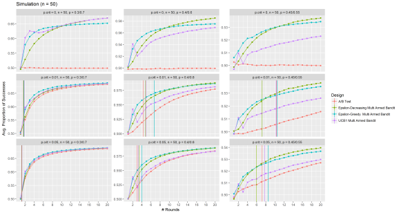
Figure: Multi Armed Bandit Simulations (n = 50)

Figure: Multi Armed Bandit Simulations (n = 500)

I performed 1,000 replications of a 20 round simulation at sample sizes of 50 and 500; critical p-value of 0%, 1% and 5%; and binomial sampling probabilities for 0.3/0.7, 0.4/0.6, and 0.45/0.55 for the two versions.

The y axis represents the proportion of successes over trails over all versions tested (which we will use as the measure of performance), and the x axis is the number of rounds. In general the performance (especially the Multi Armed Bandit methods) improves as the rounds progress.

When the critical p-value is 0%, the hypothesis test never reaches a conclusion, thus we see that the peformance of the A/B test simulations always remain at 50%, while the Multi Armed Bandit methods exploits the higher performing version thus observing increased performance.

An interesting take away is that the performance of methods diverge most when the difference in the binomial probabilites of the two versions are smaller, the critical p-value is smaller, and sample size is smaller.

Conclusion

In general I saw that the A/B test design is not optimal when it comes to maximizing the earns of the experiment, and Multi Armed Bandit methods are favorable, as expected.

The difference between A/B tests and Multi Armed Bandit tests is more prevalent when sample size is smaller, the critical p-value is smaller, and the difference in the binomial probability between the two versions are larger (p1 – p2).

The winner:

With small samples, the winner is Epsion Greedy Multi Armed Bandit, and with large samples, the winner is UCB1 Multi Armed Bandit.

Source code for the simulations are available here.