Simple Evolutionary Model Tutorial

This tutorial will demonstrate how to construct a simple evolutionary model in R. More specifically, it will show how to set up a population where individuals interact and receive payoffs according to the well known Prisoner’s dilemma, and simulate that population evolving through many generations.

The PDF of this tutorial is available here

The aim of this tutorial is to cover the basics in running evolutionary simulations in R – something that is missing in many university courses and online tutorials. The code used is simple, but demonstrates the basic use of many key functions that are useful in all circumstances. The full code is posted at the end of the tutorial. As always, it is reccomended to use RStudio for ease of code editing, problem solving, plotting etc.

Scenario

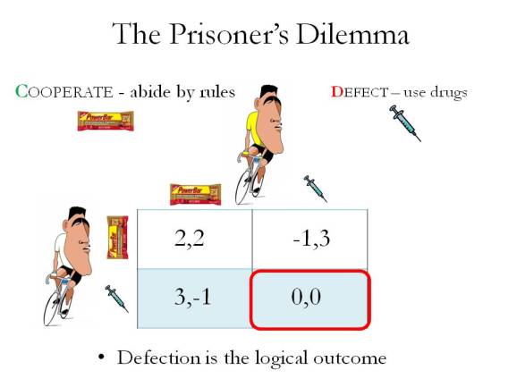
The canonical example of the game involves members of a criminal gang, but I prefer to use a more real and recent example of doping in cycling. The key to any game is players, strategies, and payoffs. In this example two cyclists can choose to cooperate by following the doping rules or defect by cheating and taking performance enhancing drugs. The average payoffs are greater if all players cooperate, but rational individuals will always defect, as they receive a higher payoff from doing so, regardless of the choice of the other player. In the cycling example it is better to cheat if the other player is cooperating, as by doing so you can win more races. It is also better to cheat if the other player is cheating, as this is required to still have a chance of competing against the enhanced other player. The outcome of this is a suboptimal scenario for everyone.

Obviously this is a simplification of the real scenario, but for more detail on the Prisoner’s dilemma in sports doping see: https://www.scientificamerican.com/article/the-doping-game-payoffs/ For anyone with a specific interest in game theory, the open course from Yale is particularly good http://oyc.yale.edu/economics/econ-159

The code

A useful first step in any code is to clear the memory using rm(list=ls()) and then set the number of generations, population size, and mutation rate.

# Clear Memory
rm(list=ls())

# Set number of generations
maxgen <- 20

# Set population size
N <- 1000

# Set the mutation rate
mutation.rate = 0.005

We can then set our payoffs, and visualise them in a dataframe. b is often used for ‘benefit’ of cooperation, and c for cost of cooperation.

# Set the payoffs
b <- 3
c <- 1

the paste function will be helpful for viewing our payoff matrix in the traditional form, with each box containing the payoffs for the two players, seperated by a comma. paste("Payoff =", b-c, sep = " ") will return the text “Payoff =” followed by whatever our value for b-c is, seperated by a space. This function becomes highly useful in more complicated settings. Here we are using it to make two vectors, x and y, which each contain the relevant payoffs for that box, seperated with a comma by the paste function. We can then name the columns C for cooperate and Dfor defect.

# visualise payoffs
x <- c(paste(b-c, b-c, sep = ", "), paste(-c, b, sep = ", "))
y <- c(paste(b, -c, sep = ", "), paste(0, 0, sep = ", "))
df <- data.frame(x,y)
colnames(df) <- c("C", "D")
rownames(df) <- colnames(df)
df
##       C     D
## C  2, 2 3, -1
## D -1, 3  0, 0

Now we can set our starting population, for which we will use all cooperators. Here we introduce the invaluable sample function. this works in the basic form of what to sample, how many, and whether to put the extracted value back in the mix. For example sample(c(1:50), 10, replace = TRUE) will sample from the numbers 1:50 ten times, and put each sample back into the mix, where it may be sampled again. In this example we are using the number 1 to mean a cooperator and -1 to mean a defecter. We can sample from a vector of just a single one (aslong as replace = TRUE) to generate a population of the right size such that all individuals will be 1 and therefore cooperators.

start <- c(1)
population <- sample(start, N, replace = TRUE)

If we wanted to start with an equal mix of cooperators and defectors we could use start <- c(1,-1) and sample from that, or if we wanted to use a certain proprtion we could use the ability of sample to make a biased sample. Here we will assign the probability 0.25 to cooperators, and 0.75 to defectors, and check the freqeuncy of our population.

start <- c(1, -1)
prob <- c(0.25, 0.75)
population <- sample(start, N, replace = TRUE, prob = prob)
length(population[population==1]) / length(population)
## [1] 0.236
length(population[population==-1]) / length(population)
## [1] 0.764

These last two lines illustrate some other simple and useful functions. length(population) will tell us how ‘long’ in individuals that vector is (or matrix row or column etc if we wanted), and can also be adapted to tell us how many of our population meet the condition of equalling one length(population[population==1]) which can be useful in extracting how frequent cooperators or defectors are in our population.

Next, we will set up a matrix to store our output from each generation. It is good practise to assign all the required rows and columns of our matrix at the start, add meaningful column names, and fill it with NA to help identify errors. output <- matrix(NA, maxgen, 4) will give us a matrix of NAs with ‘maxgen’ number of rows and 4 columns, in which we will store generation number, frequency of cooperators, freqeuncy of defectors, and average payoff.

output <- matrix(NA, maxgen, 4)
colnames(output) <- c("generation", "freq coop", "freq defect", "mean payoff")

We are now ready to open our loop. They key is to start with something (here it is our population) originally defined outside the loop, apply selection in terms of payoffs, mutations to bring in some randomness, and end up with a population at the end of the loop. Then we are ready to simply close the loop and feed back through to the start.

Simple Example Loop

A simple example loop could be constructed as follows;

# Begin Loop
for (z in 1:maxgen){
  # make two samples, to be matched as pairs of       individuals
  player1 <- sample(population,N,replace=FALSE)
  player2 <- sample(population,N,replace=FALSE)
  # make a vector for the payoff to cooperators
  coop.payoff <- 0
  # loop through the population, if player one and    player two both equal 1 (i.e. are cooperators)         assign a payoff to cooperation of b-c
  for(y in 1:N) {
   if(player1[y]==1 && player2[y]==1) {
      coop.payoff <- coop.payoff + (2 * (b - c))
   }
  }
  # After this loop, store the generation number and  payoff to cooperators in the output matrix
  output[z, 1] <- z
  output[z, 2] <- coop.payoff
}

Here, z will start at one, and go through the whole loop, and become two. This will continue until z has reached maxgen, our number of generations. Within each loop we are taking two vectors as samples of populations, which can be lined up so the first number of player 1 is partnered with the first number of player 2. We then use a second loop, going from 1 to our population size, where we use an if function to see if both players are 1 (are cooperators) and if so, we give cooperators a payoff. if(player1[y]==1 && player2[y]==1) {coop.payoff <- coop.payoff + 1} will add 1 to coop.payoff only if player1 and player2 at that place in the population (player1[2] will give the second number in player 1) both equal one.

This is obviously not a useful loop as we have not applied selection or mutation, essentially we are just seeing random variation in how many cooperators match up in each generation (and if we have a population of all 1s to begin with, this won’t change, so you can play around with the starting population)

This demonstrates the basic approach of having a loop of each generation, and nested within that having another loop that goes through each individual in the population and assigns payoffs. After the internal loop going through each individual in the payoff, the generation number (z here, as this is the letter chose for the loop of generations) and payoff are stored in the relevant part of the output matrix. The basic approach for doing this is to use something like output[z, 1] <- z which assigns row z column one to z. As we are looping through z generations, on each run through the loop output[z, 1] <- z will refer to the first row, then the second row, then the third row etc. if we wanted to view this, we could simple examine output[, 1] which will show us the first column of the matrix.

Actual Loop

As a loop has to be closed to run without error we will build up the code inside of the loop and then add the loop itself. To start we can take two vectors as samples of the population, which can be lined up so the first number of player 1 is partnered with the first number of player 2. We can then set the starting payoff as 0 for this generation.

# make pairs of individuals
  player1 <- sample(population,N,replace=FALSE)
  player2 <- sample(population,N,replace=FALSE)

# set payoff counters
  coop.payoff <- 0
  defect.payoff <- 0

Now we can prepare the internal loop where we run through the population assigning payoffs. This can be acheived with if functions for all of the possible options. These tend to run quite efficiently in R, and can be setout so if the condition is not met, the program simply moves on to the next if statement.

# Loop to calculate payoffs based on payoff matrix
   for(j in 1:N) {
    # If both players cooperate (=1) payoffs = b-c, b-c
    if(player1[j]==1 && player2[j]==1) {
      coop.payoff <- coop.payoff + (2 * (b - c))
        }
    # If player one cooperates and two defects (1, -1) payoffs = -c, b
    if(player1[j]==1 && player2[j]==-1) {
      coop.payoff <- coop.payoff - c
      defect.payoff <- defect.payoff + b
        }
     # If player two cooperates and one defects (-1, 1) payoffs = b, -c
     if(player1[j]==-1 && player2[j]==1) {
       coop.payoff <- coop.payoff - c
       defect.payoff <- defect.payoff + b
        }
     # If both players defect (-1, -1) payoffs = 0, 0
     if(player1[j]==-1 && player2[j]==-1) {
       coop.payoff <- coop.payoff + 0
       defect.payoff <- defect.payoff + 0
     }
   }

In this example we are using one vector for each strategy (coop.payoff) and (defect.payoff) that we are simply adding to or subtracting from based on the match with the other player. In this sense we are looking at payoffs to strategies rather than individuals. This is because it is much quicker to run the code this way and roughly equivalent. Sometimes it may be required to follow individual payoffs, which can be done by assigning payoff for each individual to a new vector. If this is something you are interested in, then something adapted from the code below could be useful.

player1.payoffs <- c(0)
player2.payoffs <- c(0)
for(j in 1:N) {
    # If both players cooperate (=1) payoffs = b-c, b-c
    if(player1[j]==1 && player2[j]==1) {
      player1.payoffs[j] <- b - c
      player2.payoffs[j] <- b - c
        }
}

Now that we have payoffs, we can apply selection to our population, generating a new population with the frequency of the two strategies based on their relative payoffs. In the below code we first assign any negative payoffs to 0 to allow meaningful relative payoffs to be calculated. Next, we sum the payoffs, and for strategy generate a new population based on relative payoffs. Note that we are also making our new population larger than we need to by multiplying by three. This is because we will soon be selecting a new population of 1000 for the next generation, and want to mimic some of the randomness of selection for the next generation of real scenarios, and to ensure we never end up with a decrease in population size. pop.offspring here uses the rep function, which repeats something a set number of times e.g. rep(1,5) repeats one, five times. pop.offspring therefore becomes a vector of 1s and -1s, with each strategy repeated a number of times according to their relative payoff. by sampling 1000 individuals from this new population, we have our population of selected individuals for the next generation.

# generate new population based on payoffs
  if(coop.payoff < 0){coop.payoff <- 0}
  SUM <- coop.payoff + defect.payoff
  pop.coop <- coop.payoff / SUM * N * 3
  pop.defect <- defect.payoff / SUM * N * 3
  pop.offspring <- c(rep(1,pop.coop), rep(-1,pop.defect))
  population <- sample(pop.offspring,N,replace=FALSE)
  
  # calculate frequency of cooperators and defectors in this population
  fc <- sum(population == 1) / (sum(population == 1) + sum(population == -1))
  fd <- sum(population == -1) / (sum(population == 1) + sum(population == -1))

We have also here calculated the freqeuncy of 1s and -1s in our new population, as this is what we aim to track over time.

The penultimate important step is to mutate our population. This can be done in a number of ways, but this way is the most intuitive. We define m as the number of mutations expected (mutation rate X population size). Then we use sample (it really is very useful) to pick m (here 5) numbers which represent the individuals to mutate (e.g. the 3rd, 454th, 667th, 787th and 990th). individuals at those ‘mutation places’ are then randomly given a value of -1 or 1. As such they may not actually mutate, which is something to remember when interpreting mutation rate effects.

# mutation
  m <- mutation.rate * N
  mutation.place <- sample(length(population), m, replace = FALSE)
  population[mutation.place] <- sample(c(-1, 1), 5, replace = TRUE)

In the final chunk of code we are simply recording generation number, frequency of cooperators, frequency of defectors, and average payoff in our output matrix. The last line will simply print the number of the current generation on the console. Helpful if you are running large numbers of generations and want to know how long you will be waiting!

  output[i, 1] <- i
  output[i, 2] <- fc
  output[i, 3] <- fd
  output[i, 4] <- SUM / N / 2
  print(paste("Generation =", i, sep = " "))

The loop can now be closed, so the full loop will be as follows;

# Begin Loop
for (i in 1:maxgen){
 
# make pairs of individuals
  player1 <- sample(population,N,replace=FALSE)
  player2 <- sample(population,N,replace=FALSE)

# set payoff counters
  coop.payoff <- 0
  defect.payoff <- 0
  
# Loop to calculate payoffs based on payoff matrix
   for(j in 1:N) {
    # If both players cooperate (=1) payoffs = b-c, b-c
    if(player1[j]==1 && player2[j]==1) {
      coop.payoff <- coop.payoff + (2 * (b - c))
        }
    # If player one cooperates and two defects (1, -1) payoffs = -c, b
    if(player1[j]==1 && player2[j]==-1) {
      coop.payoff <- coop.payoff - c
      defect.payoff <- defect.payoff + b
        }
     # If player two cooperates and one defects (-1, 1) payoffs = b, -c
     if(player1[j]==-1 && player2[j]==1) {
       coop.payoff <- coop.payoff - c
       defect.payoff <- defect.payoff + b
        }
     # If both players defect (-1, -1) payoffs = 0, 0
     if(player1[j]==-1 && player2[j]==-1) {
       coop.payoff <- coop.payoff + 0
       defect.payoff <- defect.payoff + 0
     }
   }
  
  # generate new population based on payoffs
  if(coop.payoff < 0){coop.payoff <- 0}
  SUM <- coop.payoff + defect.payoff
  pop.coop <- coop.payoff / SUM * N * 3
  pop.defect <- defect.payoff / SUM * N * 3
  pop.offspring <- c(rep(1,pop.coop), rep(-1,pop.defect))
  population <- sample(pop.offspring,N,replace=FALSE)
  
  # calculate frequency of cooperators and defectors in this population
  fc <- sum(population == 1) / (sum(population == 1) + sum(population == -1))
  fd <- sum(population == -1) / (sum(population == 1) + sum(population == -1))
  
  # mutation
  m <- mutation.rate * N
  mutation.place <- sample(length(population), m, replace = FALSE)
  population[mutation.place] <- sample(c(-1, 1), 5, replace = TRUE)
  
  output[i, 1] <- i
  output[i, 2] <- fc
  output[i, 3] <- fd
  output[i, 4] <- SUM / N / 2
  
  print(paste("Generation =", i, sep = " "))
 }

Plotting Figures

It is easy to visualise our results using simple plots. The online help for basic plotting is very comprehensive so I won’t bother to explain too much. Plot 1 is generation number against frequency of each strategy (cooperators in blue, defectors in red). Plot 2 is generation number against average payoff, with dotted lines for the individual options of b, b-c, 0, and -c

par(mfrow=c(2,1))
par(mar=c(4.5,4.1,1.1,1.1))
# blue = cooperators
plot(output[,1], output[,2], type = "l",lwd=2, col="blue", xlab = "generation", ylab = "frequency", ylim=c(0,1))
# red = defectors
points(output[,1], output[,3], type = "l",lwd=2, col="red")
plot(output[,1], output[,4], type = "l",lwd=2, col="black", xlab = "generation", ylab = "average payoff", ylim=c(-1,3))
abline(h = 0, lty = 3)
abline(h = (b), lty = 3, col= "green")
abline(h = (-c), lty = 3, col="red")
abline(h = (b-c), lty = 3, col="blue")

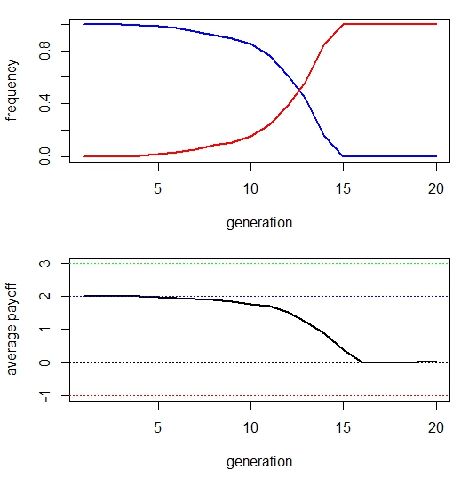
As we can see, it doesn’t take many generations for defectors to invade the population, and everyone suffers as a result.

And now we have our model. A population evolving over time, with both selection and mutation, towards the inevitable ESS outcome of defectors reaching fixation.

The full code for this model can be found below. It is easily adaptable in some ways, the benefits and costs can be changed, but if we want to make the game totally different, for example into a snowdrift game, there are some alterations that can be made. These can be found below the full script

###### Simple Prisoner's Dilemma

# Laurie Belcher 07/11/2016

# Clear Memory
rm(list=ls())

# Set number of generations
maxgen <- 20

# Set population size
N <- 1000

# Set the mutation rate
mutation.rate = 0.005

# Set the payoffs
b <- 3
c <- 1

# visualise payoffs
paste("Payoff =", b-c, sep = " ")
x <- c(paste(b-c, b-c, sep = ", "), paste(-c, b, sep = ", "))
y <- c(paste(b, -c, sep = ", "), paste(0, 0, sep = ", "))
df <- data.frame(x,y)
colnames(df) <- c("C", "D")
rownames(df) <- colnames(df)
df

# set up starting population
# -1 = will defect
# 1 = will cooperate
start <- c(1, -1)
population <- sample(start, N, replace = TRUE)
prob <- c(1, 0)
population <- sample(start, N, replace = TRUE, prob = prob)
length(population[population==1]) / length(population)
length(population[population==-1]) / length(population)


# set up matrix to store output
output <- matrix(NA, maxgen, 4)
colnames(output) <- c("generation", "freq coop", "freq defect", "mean payoff")

# Begin Loop
for (i in 1:maxgen){
 
# make pairs of individuals
  player1 <- sample(population,N,replace=FALSE)
  player2 <- sample(population,N,replace=FALSE)

# set payoff counters
  coop.payoff <- 0
  defect.payoff <- 0
  
# Loop to calculate payoffs based on payoff matrix
   for(j in 1:N) {
    # If both players cooperate (=1) payoffs = b-c, b-c
    if(player1[j]==1 && player2[j]==1) {
      coop.payoff <- coop.payoff + (2 * (b - c))
        }
    # If player one cooperates and two defects (1, -1) payoffs = -c, b
    if(player1[j]==1 && player2[j]==-1) {
      coop.payoff <- coop.payoff - c
      defect.payoff <- defect.payoff + b
        }
     # If player two cooperates and one defects (-1, 1) payoffs = b, -c
     if(player1[j]==-1 && player2[j]==1) {
       coop.payoff <- coop.payoff - c
       defect.payoff <- defect.payoff + b
        }
     # If both players defect (-1, -1) payoffs = 0, 0
     if(player1[j]==-1 && player2[j]==-1) {
       coop.payoff <- coop.payoff + 0
       defect.payoff <- defect.payoff + 0
     }
   }
  
  # generate new population based on payoffs
  if(coop.payoff < 0){coop.payoff <- 0}
  SUM <- coop.payoff + defect.payoff
  pop.coop <- coop.payoff / SUM * N * 3
  pop.defect <- defect.payoff / SUM * N * 3
  pop.offspring <- c(rep(1,pop.coop), rep(-1,pop.defect))
  population <- sample(pop.offspring,N,replace=FALSE)
  
  # calculate frequency of cooperators and defectors in this population
  fc <- sum(population == 1) / (sum(population == 1) + sum(population == -1))
  fd <- sum(population == -1) / (sum(population == 1) + sum(population == -1))
  
  # mutation
  m <- mutation.rate * N
  mutation.place <- sample(length(population), m, replace = FALSE)
  population[mutation.place] <- sample(c(-1, 1), 5, replace = TRUE)
  
  output[i, 1] <- i
  output[i, 2] <- fc
  output[i, 3] <- fd
  output[i, 4] <- SUM / N / 2
  
  print(paste("Generation =", i, sep = " "))
 }
par(mfrow=c(2,1))
par(mar=c(4.5,4.1,1.1,1.1))
# blue = cooperators
plot(output[,1], output[,2], type = "l",lwd=2, col="blue", xlab = "generation", ylab = "frequency", ylim=c(0,1))
# red = defectors
points(output[,1], output[,3], type = "l",lwd=2, col="red")
plot(output[,1], output[,4], type = "l",lwd=2, col="black", xlab = "generation", ylab = "average payoff", ylim=c(-1,3))
abline(h = 0, lty = 3)
abline(h = (b), lty = 3, col= "green")
abline(h = (-c), lty = 3, col="red")
abline(h = (b-c), lty = 3, col="blue")

Making the code more adpatable to different games

Let’s make the payoff matrix into an actual matrix. With each of the four cells referring to the playoff to player 1 (who choses between row 1 and row 2)

payoffs <- matrix(0, 2, 2)
payoffs[1,1] <- b - c
payoffs[1,2] <- -c
payoffs[2,1] <- b
payoffs[2,2] <- 0
payoffs
##      [,1] [,2]
## [1,]    2   -1
## [2,]    3    0

This is the simple prisoner’s dilemma that we have been using for the whole tutorial. Now that we are using a matrix for payoffs instead of only b and c we need to change the payoffs loop to account for this

for(j in 1:N) {
    # If both players cooperate (=1) payoffs = b-c, b-c
    if(player1[j]==1 && player2[j]==1) {
      coop.payoff <- coop.payoff + (2 * payoffs[1,1])
    }
    # If player one cooperates and two defects (1, -1) payoffs = 0, b
    if(player1[j]==1 && player2[j]==-1) {
      coop.payoff <- coop.payoff + payoffs[1,2]
      defect.payoff <- defect.payoff + payoffs[2,1]
    }
    # If player two cooperates and one defects (-1, 1) payoffs = b, 0
    if(player1[j]==-1 && player2[j]==1) {
      coop.payoff <- coop.payoff + payoffs[1,2]
      defect.payoff <- defect.payoff + payoffs[2,1]
    }
    # If both players defect (-1, -1) payoffs = -1, -1
    if(player1[j]==-1 && player2[j]==-1) {
      defect.payoff <- defect.payoff + payoffs[2,2] + payoffs[2,2]
    }
  }

The advantage of this approach is that we can easily alter the game. For example, we can change the game to a snowdrift game. The snowdrift game differs from the prisoner’s dilemma in that there is a higher payoff to cooperating with a defector than from mutual defection. This is the snowdrift payoff matrix.

payoffs <- matrix(0, 2, 2)
payoffs[1,1] <- b - c
payoffs[1,2] <- 0
payoffs[2,1] <- b
payoffs[2,2] <- -c
payoffs
##      [,1] [,2]
## [1,]    2    0
## [2,]    3   -1

If we run our model with this payoff matrix, we find a different outcome

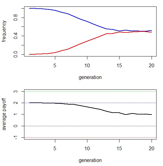
A coexistence between cooperators and defectors occurs in this scenario (though we may wish to increase the number of generations to check that this is stable). There are several other ways that the payoffs can be structured and ways that this basic model can be extended.