
cricketr sizes up legendary All-rounders of yesteryear
Want to share your content on R-bloggers? click here if you have a blog, or here if you don't.
Introduction
This is a post I have been wanting to write for several months, but had to put it off for one reason or another. In this post I use my R package cricketr to analyze the performance of All-rounder greats namely Kapil Dev, Ian Botham, Imran Khan and Richard Hadlee. All these players had talent that was natural and raw. They were good strikers of the ball and extremely lethal with their bowling. The ODI data for these players have been taken from ESPN Cricinfo.
Please be mindful of the ESPN Cricinfo Terms of Use
You can also read this post at Rpubs as cricketr-AR. Dowload this report as a PDF file from cricketr-AR
All Rounders
- Kapil Dev (Ind)
- Ian Botham (Eng)
- Imran Khan (Pak)
- Richard Hadlee (NZ)
I have sprinkled the plots with a few of my comments. Feel free to draw your conclusions! The analysis is included below
if (!require("cricketr")){
    install.packages("cricketr",)
}

library(cricketr)
The data for any particular ODI player can be obtained with the getPlayerDataOD() function. To do you will need to go to ESPN CricInfo Playerand type in the name of the player for e.g Kapil Dev, etc. This will bring up a page which have the profile number for the player e.g. for Kapil Dev this would be http://www.espncricinfo.com/india/content/player/30028.html. Hence, Kapils’s profile is 30028. This can be used to get the data for Kapil Dev’s data as shown below. I have already executed the below 4 commands and I will use the files to run further commands
#kapil1 <- getPlayerDataOD(30028,dir="..",file="kapil1.csv",type="batting")
#botham11 <- getPlayerDataOD(9163,dir="..",file="botham1.csv",type="batting")
#imran1 <- getPlayerDataOD(40560,dir="..",file="imran1.csv",type="batting")
#hadlee1 <- getPlayerDataOD(37224,dir="..",file="hadlee1.csv",type="batting")
Analyses of batting performances of the All Rounders
The following plots gives the analysis of the 4 ODI batsmen
- Kapil Dev (Ind) – Innings – 225, Runs = 3783, Average=23.79, Strike Rate= 95.07
- Ian Botham (Eng) – Innings – 116, Runs= 2113, Average=23.21, Strike Rate= 79.10
- Imran Khan (Pak) – Innings – 175, Runs= 3709, Average=33.41, Strike Rate= 72.65
- Richard Hadlee (NZ) – Innings – 115, Runs= 1751, Average=21.61, Strike Rate= 75.50
Plot of 4s, 6s and the scoring rate in ODIs
The 3 charts below give the number of
- 4s vs Runs scored
- 6s vs Runs scored
- Balls faced vs Runs scored
A regression line is fitted in each of these plots for each of the ODI batsmen
A. Kapil Dev
It can be seen that Kapil scores four 4’s when he scores 50. Also after facing 50 deliveries he scores around 43
par(mfrow=c(1,3))
par(mar=c(4,4,2,2))
batsman4s("./kapil1.csv","Kapil")
batsman6s("./kapil1.csv","Kapil")
batsmanScoringRateODTT("./kapil1.csv","Kapil")

dev.off()
## null device
##           1
B. Ian Botham
Botham scores around 39 runs after 50 deliveries
par(mfrow=c(1,3))
par(mar=c(4,4,2,2))
batsman4s("./botham1.csv","Botham")
batsman6s("./botham1.csv","Botham")
batsmanScoringRateODTT("./botham1.csv","Botham")

dev.off()
## null device
##           1
C. Imran Khan
Imran scores around 36 runs for 50 deliveries
par(mfrow=c(1,3))
par(mar=c(4,4,2,2))
batsman4s("./imran1.csv","Imran")
batsman6s("./imran1.csv","Imran")
batsmanScoringRateODTT("./imran1.csv","Imran")

dev.off()
## null device
##           1
D. Richard Hadlee
Hadlee also scores around 30 runs facing 50 deliveries
par(mfrow=c(1,3))
par(mar=c(4,4,2,2))
batsman4s("./hadlee1.csv","Hadlee")
batsman6s("./hadlee1.csv","Hadlee")
batsmanScoringRateODTT("./hadlee1.csv","Hadlee")

dev.off()
## null device
##           1
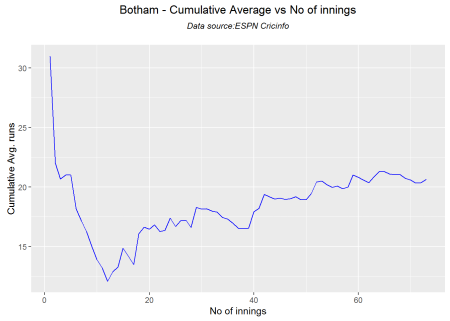
Cumulative Average runs of batsman in career
Kapils cumulative avrerage runs drops towards the last 15 innings wheres Botham had a good run towards the end of his career. Imran performance as a batsman really peaks towards the end with a cumulative average of almost 25 runs. Hadlee has a stead performance
par(mfrow=c(2,2))
par(mar=c(4,4,2,2))
batsmanCumulativeAverageRuns("./kapil1.csv","Kapil")

batsmanCumulativeAverageRuns("./botham1.csv","Botham")
batsmanCumulativeAverageRuns("./imran1.csv","Imran")

batsmanCumulativeAverageRuns("./hadlee1.csv","Hadlee")

dev.off()
## null device
##           1
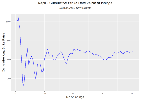
Cumulative Average strike rate of batsman in career
Kapil’s strike rate is superlative touching the 90’s steadily. Botham’s strike drops dramatically towards the latter part of his career. Imran average at a steady 75 and Hadlee averages around 85.
par(mfrow=c(2,2))
par(mar=c(4,4,2,2))
batsmanCumulativeStrikeRate("./kapil1.csv","Kapil")
batsmanCumulativeStrikeRate("./botham1.csv","Botham")

batsmanCumulativeStrikeRate("./imran1.csv","Imran")

batsmanCumulativeStrikeRate("./hadlee1.csv","Hadlee")

dev.off()
## null device
##           1
Relative Mean Strike Rate
Kapil tops the strike rate among all the all-rounders. This is really a revelation to me. This can also be seen in the original data in Kapil’s strike rate is at a whopping 95.07 in comparison to Botham, Inran and Hadlee who are at 79.1,72.65 and 75.50 respectively
par(mar=c(4,4,2,2))
frames <- list("./kapil1.csv","./botham1.csv","imran1.csv","hadlee1.csv")
names <- list("Kapil","Botham","Imran","Hadlee")
relativeBatsmanSRODTT(frames,names)

Relative Runs Frequency Percentage
This plot shows that Imran has a much better average runs scored over the other all rounders followed by Kapil
frames <- list("./kapil1.csv","./botham1.csv","imran1.csv","hadlee1.csv")
names <- list("Kapil","Botham","Imran","Hadlee")
relativeRunsFreqPerfODTT(frames,names)

Relative cumulative average runs in career
It can be seen clearly that Imran Khan leads the pack in cumulative average runs followed by Kapil Dev and then Botham
frames <- list("./kapil1.csv","./botham1.csv","imran1.csv","hadlee1.csv")
names <- list("Kapil","Botham","Imran","Hadlee")
relativeBatsmanCumulativeAvgRuns(frames,names)

Relative cumulative average strike rate in career
In the cumulative strike rate Hadlee and Kapil run a close race.
frames <- list("./kapil1.csv","./botham1.csv","imran1.csv","hadlee1.csv")
names <- list("Kapil","Botham","Imran","Hadlee")
relativeBatsmanCumulativeStrikeRate(frames,names)

Percent 4’s,6’s in total runs scored
The plot below shows the contrib
frames <- list("./kapil1.csv","./botham1.csv","imran1.csv","hadlee1.csv")
names <- list("Kapil","Botham","Imran","Hadlee")
runs4s6s <-batsman4s6s(frames,names)

print(runs4s6s)
##                Kapil Botham Imran Hadlee
## Runs(1s,2s,3s) 72.08  66.53 77.53  73.27
## 4s             21.98  25.78 17.61  21.08
## 6s              5.94   7.68  4.86   5.65
Runs forecast
The forecast for the batsman is shown below.
par(mfrow=c(2,2))
par(mar=c(4,4,2,2))
batsmanPerfForecast("./kapil1.csv","Kapil")
batsmanPerfForecast("./botham1.csv","Botham")
batsmanPerfForecast("./imran1.csv","Imran")
batsmanPerfForecast("./hadlee1.csv","Hadlee")

dev.off()
## null device
##           1
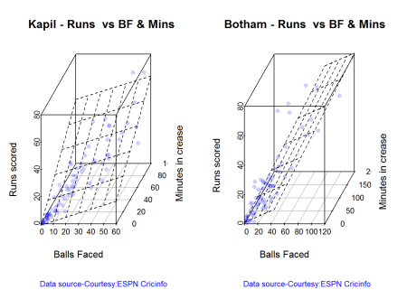
3D plot of Runs vs Balls Faced and Minutes at Crease
The plot is a scatter plot of Runs vs Balls faced and Minutes at Crease. A prediction plane is fitted
par(mfrow=c(1,2))
par(mar=c(4,4,2,2))
battingPerf3d("./kapil1.csv","Kapil")
battingPerf3d("./botham1.csv","Botham")
dev.off()
## null device
##           1
par(mfrow=c(1,2))
par(mar=c(4,4,2,2))
battingPerf3d("./imran1.csv","Imran")
battingPerf3d("./hadlee1.csv","Hadlee")

dev.off()
## null device
##           1
Predicting Runs given Balls Faced and Minutes at Crease
A multi-variate regression plane is fitted between Runs and Balls faced +Minutes at crease.
BF <- seq( 10, 200,length=10)
Mins <- seq(30,220,length=10)
newDF <- data.frame(BF,Mins)

kapil <- batsmanRunsPredict("./kapil1.csv","Kapil",newdataframe=newDF)
botham <- batsmanRunsPredict("./botham1.csv","Botham",newdataframe=newDF)
imran <- batsmanRunsPredict("./imran1.csv","Imran",newdataframe=newDF)
hadlee <- batsmanRunsPredict("./hadlee1.csv","Hadlee",newdataframe=newDF)
The fitted model is then used to predict the runs that the batsmen will score for a hypotheticial Balls faced and Minutes at crease. It can be seen that Kapil is the best bet for a balls faced and minutes at crease followed by Botham.
batsmen <-cbind(round(kapil$Runs),round(botham$Runs),round(imran$Runs),round(hadlee$Runs))
colnames(batsmen) <- c("Kapil","Botham","Imran","Hadlee")
newDF <- data.frame(round(newDF$BF),round(newDF$Mins))
colnames(newDF) <- c("BallsFaced","MinsAtCrease")
predictedRuns <- cbind(newDF,batsmen)
predictedRuns
##    BallsFaced MinsAtCrease Kapil Botham Imran Hadlee
## 1          10           30    16      6    10     15
## 2          31           51    33     22    22     28
## 3          52           72    49     38    33     42
## 4          73           93    65     54    45     56
## 5          94          114    81     70    56     70
## 6         116          136    97     86    67     84
## 7         137          157   113    102    79     97
## 8         158          178   130    117    90    111
## 9         179          199   146    133   102    125
## 10        200          220   162    149   113    139
Highest runs likelihood
The plots below the runs likelihood of batsman. This uses K-Means . A. Kapil Dev
batsmanRunsLikelihood("./kapil1.csv","Kapil")

## Summary of  Kapil 's runs scoring likelihood
## **************************************************
##
## There is a 34.57 % likelihood that Kapil  will make  22 Runs in  24 balls over 34  Minutes
## There is a 17.28 % likelihood that Kapil  will make  46 Runs in  46 balls over  65  Minutes
## There is a 48.15 % likelihood that Kapil  will make  5 Runs in  7 balls over 9  Minutes
B. Ian Botham
batsmanRunsLikelihood("./botham1.csv","Botham")

## Summary of  Botham 's runs scoring likelihood
## **************************************************
##
## There is a 47.95 % likelihood that Botham  will make  9 Runs in  12 balls over 15  Minutes
## There is a 39.73 % likelihood that Botham  will make  23 Runs in  32 balls over  44  Minutes
## There is a 12.33 % likelihood that Botham  will make  59 Runs in  74 balls over 101  Minutes
C. Imran Khan
batsmanRunsLikelihood("./imran1.csv","Imran")

## Summary of  Imran 's runs scoring likelihood
## **************************************************
##
## There is a 23.33 % likelihood that Imran  will make  36 Runs in  54 balls over 74  Minutes
## There is a 60 % likelihood that Imran  will make  14 Runs in  18 balls over  23  Minutes
## There is a 16.67 % likelihood that Imran  will make  53 Runs in  90 balls over 115  Minutes
D. Richard Hadlee
batsmanRunsLikelihood("./hadlee1.csv","Hadlee")

## Summary of  Hadlee 's runs scoring likelihood
## **************************************************
##
## There is a 6.1 % likelihood that Hadlee  will make  64 Runs in  79 balls over 90  Minutes
## There is a 42.68 % likelihood that Hadlee  will make  25 Runs in  33 balls over  44  Minutes
## There is a 51.22 % likelihood that Hadlee  will make  9 Runs in  11 balls over 15  Minutes
Average runs at ground and against opposition
A. Kapil Dev
par(mfrow=c(1,2))
par(mar=c(4,4,2,2))
batsmanAvgRunsGround("./kapil1.csv","Kapil")
batsmanAvgRunsOpposition("./kapil1.csv","Kapil")

dev.off()
## null device
##           1
B. Ian Botham
par(mfrow=c(1,2))
par(mar=c(4,4,2,2))
batsmanAvgRunsGround("./botham1.csv","Botham")
batsmanAvgRunsOpposition("./botham1.csv","Botham")

dev.off()
## null device
##           1
C. Imran Khan
par(mfrow=c(1,2))
par(mar=c(4,4,2,2))
batsmanAvgRunsGround("./imran1.csv","Imran")
batsmanAvgRunsOpposition("./imran1.csv","Imran")

dev.off()
## null device
##           1
D. Richard Hadlee
par(mfrow=c(1,2))
par(mar=c(4,4,2,2))
batsmanAvgRunsGround("./hadlee1.csv","Hadlee")
batsmanAvgRunsOpposition("./hadlee1.csv","Hadlee")

dev.off()
## null device
##           1
Moving Average of runs over career
The moving average for the 4 batsmen indicate the following
Kapil’s performance drops significantly while there is a slump in Botham’s performance. On the other hand Imran and Hadlee’s performance were on the upswing.
par(mfrow=c(2,2))
par(mar=c(4,4,2,2))
batsmanMovingAverage("./kapil1.csv","Kapil")
batsmanMovingAverage("./botham1.csv","Botham")
batsmanMovingAverage("./imran1.csv","Imran")
batsmanMovingAverage("./hadlee1.csv","Hadlee")

dev.off()
## null device
##           1
Check batsmen in-form, out-of-form
[1] “**************************** Form status of Kapil ****************************\n\n
Population size: 72
Mean of population: 19.38 \n
Sample size: 9 Mean of sample: 6.78 SD of sample: 6.14 \n\n
Null hypothesis H0 : Kapil ‘s sample average is within 95% confidence interval of population average\n
Alternative hypothesis Ha : Kapil ‘s sample average is below the 95% confidence interval of population average\n\n
Kapil ‘s Form Status: Out-of-Form because the p value: 8.4e-05 is less than alpha= 0.05
“**************************** Form status of Botham ****************************\n\n
Population size: 65
Mean of population: 21.29 \n
Sample size: 8 Mean of sample: 15.38 SD of sample: 13.19 \n\n
Null hypothesis H0 : Botham ‘s sample average is within 95% confidence interval of population average\n
Alternative hypothesis Ha : Botham ‘s sample average is below the 95% confidence interval of population average\n\n
Botham ‘s Form Status: In-Form because the p value: 0.120342 is greater than alpha= 0.05 \n
“**************************** Form status of Imran ****************************\n\n
Population size: 54
Mean of population: 24.94 \n
Sample size: 6 Mean of sample: 30.83 SD of sample: 25.4 \n\n
Null hypothesis H0 : Imran ‘s sample average is within 95% confidence interval of population average\n
Alternative hypothesis Ha : Imran ‘s sample average is below the 95% confidence interval of population average\n\n
Imran ‘s Form Status: In-Form because the p value: 0.704683 is greater than alpha= 0.05 \n
“**************************** Form status of Hadlee ****************************\n\n
Population size: 73
Mean of population: 18 \n
Sample size: 9 Mean of sample: 27 SD of sample: 24.27 \n\n
Null hypothesis H0 : Hadlee ‘s sample average is within 95% confidence interval of population average\n
Alternative hypothesis Ha : Hadlee ‘s sample average is below the 95% confidence interval of population average\n\n
Hadlee ‘s Form Status: In-Form because the p value: 0.85262 is greater than alpha= 0.05 \n *******************************************************************************************\n\n”
Analyses of bowling performances of the All Rounders
The following plots gives the analysis of the 4 ODI batsmen
- Kapil Dev (Ind) – Innings – 225, Wickets = 253, Average=27.45, Economy Rate= 3.71
- Ian Botham (Eng) – Innings – 116, Wickets = 145, Average=28.54, Economy Rate= 3.96
- Imran Khan (Pak) – Innings – 175, Wickets = 182, Average=26.61, Economy Rate= 3.89
- Richard Hadlee (NZ) – Innings – 115, Wickets = 158, Average=21.56, Economy Rate= 3.30
Botham has the highest number of innings and wickets followed closely by Mitchell. Imran and Hadlee have relatively fewer innings.
To get the bowler’s data use
#kapil2 <- getPlayerDataOD(30028,dir="..",file="kapil2.csv",type="bowling")
#botham2 <- getPlayerDataOD(9163,dir="..",file="botham2.csv",type="bowling")
#imran2 <- getPlayerDataOD(40560,dir="..",file="imran2.csv",type="bowling")
#hadlee2 <- getPlayerDataOD(37224,dir="..",file="hadlee2.csv",type="bowling")
“`
Wicket Frequency percentage
This plot gives the percentage of wickets for each wickets (1,2,3…etc).
par(mfrow=c(1,4))
par(mar=c(4,4,2,2))
bowlerWktsFreqPercent("./kapil2.csv","Kapil")
bowlerWktsFreqPercent("./botham2.csv","Botham")
bowlerWktsFreqPercent("./imran2.csv","Imran")
bowlerWktsFreqPercent("./hadlee2.csv","Hadlee")

dev.off()
## null device
##           1
Wickets Runs plot
The plot below gives a boxplot of the runs ranges for each of the wickets taken by the bowlers.
par(mfrow=c(1,4))
par(mar=c(4,4,2,2))

bowlerWktsRunsPlot("./kapil2.csv","Kapil")
bowlerWktsRunsPlot("./botham2.csv","Botham")
bowlerWktsRunsPlot("./imran2.csv","Imran")
bowlerWktsRunsPlot("./hadlee2.csv","Hadlee")

dev.off()
## null device
##           1
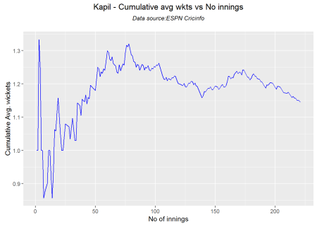
Cumulative average wicket plot
Botham has the best cumulative average wicket touching almost 1.6 wickets followed by Hadlee
par(mfrow=c(1,3))
par(mar=c(4,4,2,2))
bowlerCumulativeAvgWickets("./kapil2.csv","Kapil")
bowlerCumulativeAvgWickets("./botham2.csv","Botham")

bowlerCumulativeAvgWickets("./imran2.csv","Imran")

bowlerCumulativeAvgWickets("./hadlee2.csv","Hadlee")

dev.off()
## null device
##           1
par(mfrow=c(1,3))
par(mar=c(4,4,2,2))
bowlerCumulativeAvgEconRate("./kapil2.csv","Kapil")

bowlerCumulativeAvgEconRate("./botham2.csv","Botham")

bowlerCumulativeAvgEconRate("./imran2.csv","Imran")

bowlerCumulativeAvgEconRate("./hadlee2.csv","Hadlee")

dev.off()
## null device
##           1
Average wickets in different grounds and opposition
A. Kapil Dev
par(mfrow=c(1,2))
par(mar=c(4,4,2,2))
bowlerAvgWktsGround("./kapil2.csv","Kapil")
bowlerAvgWktsOpposition("./kapil2.csv","Kapil")

dev.off()
## null device
##           1
B. Ian Botham
par(mfrow=c(1,2))
par(mar=c(4,4,2,2))
bowlerAvgWktsGround("./botham2.csv","Botham")
bowlerAvgWktsOpposition("./botham2.csv","Botham")

dev.off()
## null device
##           1
C. Imran Khan
par(mfrow=c(1,2))
par(mar=c(4,4,2,2))
bowlerAvgWktsGround("./imran2.csv","Imran")
bowlerAvgWktsOpposition("./imran2.csv","Imran")

dev.off()
## null device
##           1
D. Richard Hadlee
par(mfrow=c(1,2))
par(mar=c(4,4,2,2))
bowlerAvgWktsGround("./hadlee2.csv","Hadlee")
bowlerAvgWktsOpposition("./hadlee2.csv","Hadlee")

dev.off()
## null device
##           1
Relative bowling performance
It can be seen that Botham is the most effective wicket taker of the lot
frames <- list("./kapil2.csv","./botham2.csv","imran2.csv","hadlee2.csv")
names <- list("Kapil","Botham","Imran","Hadlee")
relativeBowlingPerf(frames,names)

Relative Economy Rate against wickets taken
Hadlee has the best overall economy rate followed by Kapil Dev
frames <- list("./kapil2.csv","./botham2.csv","imran2.csv","hadlee2.csv")
names <- list("Kapil","Botham","Imran","Hadlee")
relativeBowlingERODTT(frames,names)

Relative cumulative average wickets of bowlers in career
This plot confirms the wicket taking ability of Botham followed by Hadlee
frames <- list("./kapil2.csv","./botham2.csv","imran2.csv","hadlee2.csv")
names <- list("Kapil","Botham","Imran","Hadlee")
relativeBowlerCumulativeAvgWickets(frames,names)

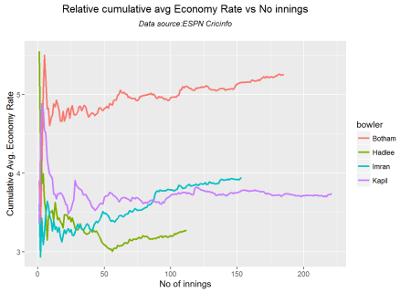
Relative cumulative average economy rate of bowlers
frames <- list("./kapil2.csv","./botham2.csv","imran2.csv","hadlee2.csv")
names <- list("Kapil","Botham","Imran","Hadlee")
relativeBowlerCumulativeAvgEconRate(frames,names)
Moving average of wickets over career
This plot shows that Hadlee has the best economy rate followed by Kapil
par(mfrow=c(2,2))
par(mar=c(4,4,2,2))
bowlerMovingAverage("./kapil2.csv","Kapil")
bowlerMovingAverage("./botham2.csv","Botham")
bowlerMovingAverage("./imran2.csv","Imran")
bowlerMovingAverage("./hadlee2.csv","Hadlee")

dev.off()
## null device
##           1
Wickets forecast
par(mfrow=c(2,2))
par(mar=c(4,4,2,2))
bowlerPerfForecast("./kapil2.csv","Kapil")
bowlerPerfForecast("./botham2.csv","Botham")
bowlerPerfForecast("./imran2.csv","Imran")
bowlerPerfForecast("./hadlee2.csv","Hadlee")

dev.off()
## null device
##           1
Check bowler in-form, out-of-form
“**************************** Form status of Kapil ****************************\n\n
Population size: 198
Mean of population: 1.2 \n Sample size: 23 Mean of sample: 0.65 SD of sample: 0.83 \n\n
Null hypothesis H0 : Kapil ‘s sample average is within 95% confidence interval \n of population average\n
Alternative hypothesis Ha : Kapil ‘s sample average is below the 95% confidence\n interval of population average\n\n
Kapil ‘s Form Status: Out-of-Form because the p value: 0.002097 is less than alpha= 0.05 \n
“**************************** Form status of Botham ****************************\n\n
Population size: 166
Mean of population: 1.58 \n Sample size: 19 Mean of sample: 1.47 SD of sample: 1.12 \n\n
Null hypothesis H0 : Botham ‘s sample average is within 95% confidence interval \n of population average\n
Alternative hypothesis Ha : Botham ‘s sample average is below the 95% confidence\n interval of population average\n\n
Botham ‘s Form Status: In-Form because the p value: 0.336694 is greater than alpha= 0.05 \n
“**************************** Form status of Imran ****************************\n\n
Population size: 137
Mean of population: 1.23 \n Sample size: 16 Mean of sample: 0.81 SD of sample: 0.91 \n\n
Null hypothesis H0 : Imran ‘s sample average is within 95% confidence interval \n of population average\n
Alternative hypothesis Ha : Imran ‘s sample average is below the 95% confidence\n interval of population average\n\n
Imran ‘s Form Status: Out-of-Form because the p value: 0.041727 is less than alpha= 0.05 \n
“**************************** Form status of Hadlee ****************************\n\n
Population size: 100
Mean of population: 1.38 \n Sample size: 12 Mean of sample: 1.67 SD of sample: 1.37 \n\n
Null hypothesis H0 : Hadlee ‘s sample average is within 95% confidence interval \n of population average\n
Alternative hypothesis Ha : Hadlee ‘s sample average is below the 95% confidence\n interval of population average\n\n
Hadlee ‘s Form Status: In-Form because the p value: 0.761265 is greater than alpha= 0.05 \n *******************************************************************************************\n\n”
Key findings
Here are some key conclusions ODI batsmen
- Kapil Dev’s strike rate stands high above the other 3
- Imran Khan has the best cumulative average runs followed by Kapil
- Botham is the most effective wicket taker followed by Hadlee
- Hadlee is the most economical bowler and is followed by Kapil Dev
- For a hypothetical Balls Faced and Minutes at creases Kapil will score the most runs followed by Botham
- The moving average of indicates that the best is yet to come for Imran and Hadlee. Kapil and Botham were on the decline
Also see my other posts in R
- A primer on Qubits, Quantum gates abd Quantum operations
- Deblurring with OpenCV:Weiner filter reloaded
- Designing a Social Web Portal
- A crime map of India in R – Crimes against women
- Bend it like Bluemix, MongoDB with autoscaling – Part 2
- Mirror, mirror . the best batsman of them all?
For a full list of posts see Index of posts

R-bloggers.com offers daily e-mail updates about R news and tutorials about learning R and many other topics. Click here if you're looking to post or find an R/data-science job.
Want to share your content on R-bloggers? click here if you have a blog, or here if you don't.