I came across a local website where individuals/dealers in Malaysia can post information on used and new cars that they are selling. Why i, in particular, would browse such a site might dumbfound some people (those who personally know me would know what i’m talking about), i nevertheless found myself spending over an hour going through the posts put up my hundreds of users in Malaysia; and it got me wondering. It would be pretty interesting to explore these posts a little further by extracting the information from the site.

The website that i was referring to is carlist.my, which they claim is:

…Malaysia’s No.1 car site connecting car buyers, sellers and enthusiasts to a single platform which encompasses car classifieds and informative content.

Similar to the property data scraping post, i figured it would be best to limit the scraping to a particular categorical variable; in this case, a specific car manufacturer. I chose Perodua since i’ve noticed that most Malaysians consider it the more popular half of the two manufacturers that dominate the local market.

Alright, now that the manufacturer has been chosen, it’s time to study the site a little bit so that the code can accommodate for the site’s idiosyncrasies.

From the site’s search results page, i see that there are 12 search results per page. So going through 250 search result pages should give me all the links to 3000 car sale information, and navigating to these links should provide me with the information i need for each sale.

Seeing how i want to retrieve data for both used and new car sales, i’ve decided to run the code twice, once for the new cars URL and once for the used cars URL.

In contrast to what i did in the property data post, i decided to place the loops in a function and then assign the result of that function to a variable. The PC i was using had an Intel i3-4150 processor with a 4GB RAM and using a 5Mbps connection, on WiFi. Needless to say, it took an eternity, but that didn’t bother me. What did bother me was that it also ends with the computer crashing because of all the memory it takes to hold that information. Tried again on an i5-5200 computer with an 8GB RAM, same internet connection but this time using an ethernet cable (helplessly hoping that this would make a difference). It still took eons to complete, but at least it didn’t crash.

The link for the code i used is below. As a note, the site_first variable is where the URL for the search results page needs to be pasted, minus the page number.

#load libraries
library(stringr)
library(rvest)
library(ggvis)
library(dplyr)
library(ggplot2)

#The site
Site = "http://www.carlist.my/"

#The first half of the URL..
#Here you can paste the URL of the search results; used or new 
site_first = "http://www.carlist.my/used-cars/perodua?page_number=" 
  
#concatenate them together, with the coerced digit in between them. This digit is the page number
siteCom = paste(site_first, as.character(1), sep = "")
siteLocHTML = html(siteCom)

#Assign the links of the first page to x and y
siteLocHTML %>% html_nodes(".js-vr38dett-title") %>% 
  html_text() %>% data.frame() -> x

siteLocHTML %>% html_nodes(".js-vr38dett-title") %>% 
  html_attr("href") %>% data.frame() -> y

#Create function that will loop through the second page and onwards
Links = function(limit){
  
  for(i in 2:limit){
    
    siteCom = paste(site_first, as.character(i), sep = "")
    siteLocHTML = html(siteCom)
    
    siteLocHTML %>% html_nodes(".js-vr38dett-title") %>% 
      html_text() %>% data.frame() -> x_next
    
    siteLocHTML %>% html_nodes(".js-vr38dett-title") %>% 
      html_attr("href") %>% data.frame() -> y_next
    
    x = rbind(x, x_next)
    y = rbind(y, y_next)
    
  }

z = cbind(x,y)
return(z)
}

complete = Links(250) #The 250 represents the search pages
rm(x,y)

for(i in 3:12){
  complete[,i] = NA
}

headers = c("Desc", "Link", "Make", "Model", "Year", "Engine.Cap", "Transm", "Mileage", "Color", "Car.Type", "Updated", "Price")

names(complete) = headers

write.csv(complete, "Links_CarList_Used.csv", row.names = FALSE) #export the links, for backup

Details = function(dataframe, i){

  for(j in 1:nrow(dataframe)){  
  
        link = html(paste(Site, dataframe[j, i], sep = ""))
        
        link %>% html_nodes("#single-post-detail") %>% 
          html_nodes(".section-body") %>% 
          html_nodes(".row-fluid") %>% 
          html_nodes(".span6") %>% 
          html_nodes(".list") %>% 
          html_nodes(".tr-make") %>% 
          html_nodes(".data") %>% 
          html_text() -> a
        
        a = str_replace_all(a, "\n", "")
        a = str_replace_all(a, " ", "")
        
          dataframe[j,"Make"] = a
        
        link %>% html_nodes("#single-post-detail") %>% 
          html_nodes(".section-body") %>% 
          html_nodes(".row-fluid") %>% 
          html_nodes(".span6") %>% 
          html_nodes(".list") %>% 
          html_nodes(".tr-model") %>% 
          html_nodes(".data") %>% 
          html_text() -> a
        
        a = str_replace_all(a, "\n", "")
        a = str_replace_all(a, " ", "")
        
        dataframe[j,"Model"] = a
        
        link %>% html_nodes("#single-post-detail") %>% 
          html_nodes(".section-body") %>% 
          html_nodes(".row-fluid") %>% 
          html_nodes(".span6") %>% 
          html_nodes(".list") %>% 
          html_nodes(".tr-year") %>% 
          html_nodes(".data") %>% 
          html_text() -> a
        
        a = str_replace_all(a, "\n", "")
        a = str_replace_all(a, " ", "")
        
        dataframe[j,"Year"] = a
        
        link %>% html_nodes("#single-post-detail") %>% 
          html_nodes(".section-body") %>% 
          html_nodes(".row-fluid") %>% 
          html_nodes(".span6") %>% 
          html_nodes(".list") %>% 
          html_nodes(".tr-engine") %>% 
          html_nodes(".data") %>% 
          html_text() -> a
        
        a = str_replace_all(a, "\n", "")
        a = str_replace_all(a, " ", "")
        
        dataframe[j,"Engine.Cap"] = a
        
        link %>% html_nodes("#single-post-detail") %>% 
          html_nodes(".section-body") %>% 
          html_nodes(".row-fluid") %>% 
          html_nodes(".span6") %>% 
          html_nodes(".list") %>% 
          html_nodes(".tr-transmission") %>% 
          html_nodes(".data") %>% 
          html_text() -> a
        
        a = str_replace_all(a, "\n", "")
        a = str_replace_all(a, " ", "")
        
        dataframe[j,"Transm"] = a
        
        link %>% html_nodes("#single-post-detail") %>% 
          html_nodes(".section-body") %>% 
          html_nodes(".row-fluid") %>% 
          html_nodes(".span6") %>% 
          html_nodes(".list") %>% 
          html_nodes(".tr-mileage") %>% 
          html_nodes(".data") %>% 
          html_text() -> a
        
        a = str_replace_all(a, "\n", "")
        a = str_replace_all(a, "  ", "")
        
        dataframe[j,"Mileage"] = a
        
        link %>% html_nodes("#single-post-detail") %>% 
          html_nodes(".section-body") %>% 
          html_nodes(".row-fluid") %>% 
          html_nodes(".span6") %>% 
          html_nodes(".list") %>% 
          html_nodes(".tr-color") %>% 
          html_nodes(".data") %>% 
          html_text() -> a
        
        a = str_replace_all(a, "\n", "")
        a = str_replace_all(a, " ", "")
        
        dataframe[j,"Color"] = a
        
        link %>% html_nodes("#single-post-detail") %>% 
          html_nodes(".section-body") %>% 
          html_nodes(".row-fluid") %>% 
          html_nodes(".span6") %>% 
          html_nodes(".list") %>% 
          html_nodes(".tr-car-type") %>% 
          html_nodes(".data") %>% 
          html_text() -> a
        
        a = str_replace_all(a, "\n", "")
        a = str_replace_all(a, " ", "")
        
        dataframe[j,"Car.Type"] = a
        
        link %>% html_nodes("#single-post-detail") %>% 
          html_nodes(".section-body") %>% 
          html_nodes(".row-fluid") %>% 
          html_nodes(".span6") %>% 
          html_nodes(".list") %>% 
          html_nodes(".tr-updated") %>% 
          html_nodes(".data") %>% 
          html_text() -> a
        
        a = str_replace_all(a, "\n", "")
        #a = str_replace_all(a, " ", "")
        
        dataframe[j,"Updated"] = a
        

        link %>% html_nodes("#single-post-header") %>% 
          html_nodes(".post-highlight") %>% 
          html_nodes(".price") %>% 
          html_text() -> a
        
        a = str_replace_all(a, "\n", "")
        a = str_replace_all(a, " ", "")
        
        dataframe[j,"Price"] = a
        
}

return(dataframe)

}

Final = Details(complete, 2)
write.csv(Final, "Final_CarList_Used.csv", row.names = FALSE)

The information that was extracted for each post are listed below, with the column name in paratheses:
1. Description of the post (Desc)
2. Link to the post (Link)
3. Manufacturer name (Make)
4. Car model (Model)
5. Year of the model (Year)
6. Engine’s capacity (Engine.Cap)
7. Transmission (Transm)
8. Mileage (Mileage)
9. Color (Color)
10. New or Used (Car.Type)
11. Date post was updated (Updated)
12. Price of the car (Price)

And that brings us to the most tedious part of the whole activity: cleaning the data and re-classification.

As it stands, all the variables are of class character, but the way i see it is that only the first two should be remain that way. Price and Mileage should be converted to integers while Model, Year, Transm, Car.Type, Color and Engine.Cap should be factors; and Year into POSIXct.

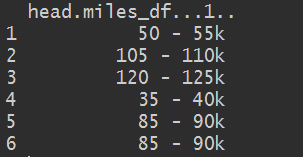
Changing the class of each variable wasn’t so much of an issue, except in the case of Mileage. On the site, Mileages are either stated as, for instance, “95,000”; or as a range, such as “95 – 105k km”. The format for the former wasn’t much trouble as it only involved having to remove the comma, and then coercing the class to integer using as.integer(). The issue lied in the posts that contain ranges. In order to have a nice tidy format, i decided to average the mileages that were posted (whether this is acceptable, however, i’m not sure). This means isolating both ends of the range in separate columns and then using dplyr’s mutate() function to create a new variable. The code is below:

miles = compiled_fac[, "Mileage"]

#Remove "km" from all observations
miles = str_replace_all(miles, "km", "")

#Isolate observations that have "k" in a separate dataframe
miles_df = data.frame(miles[grep("k", miles)])

#Add two columns to this new df
miles_df[,"Start"] = NA
miles_df[,"Stop"] = NA



for(i in 1: nrow(miles_df)){
  
  #To assign the location of the hyphen in string
  limit = as.integer(gregexpr(" - ", miles_df[i,1]))
  
  #Extract only lower end of the range and assign to Start column
  miles_df[i, "Start"] = substr(miles_df[i,1], 0, limit - 1)
  
  #Extract only higher end of the range and assign to Stop column
  miles_df[i, "Stop"] = substr(miles_df[i,1], 
                               as.integer(gregexpr(" - ", miles_df[i,1])) + 3, 
                               nchar(as.character(miles_df[i,1])))
  
}

#Remove the "k" from lower end
miles_df[, "Stop"] = str_replace_all(miles_df[,"Stop"], "k ", "")

#check if any NAs
anyNA(as.integer(miles_df[, "Stop"])) 
anyNA(as.integer(miles_df[, "Start"]))

#Prepare columns for calculation
miles_df[,"Start"] = as.integer(miles_df[,"Start"])
miles_df[,"Stop"] = as.integer(miles_df[,"Stop"])


dplyr::mutate(miles_df, avg_miles = ((Start + Stop)/2)*1000) -> miles_df_adj
new_miles = miles_df_adj$avg_miles

miles[grep("k", miles)] = new_miles

miles = as.integer(str_replace_all(miles, ",", ""))

compiled_fac[,"Mileage"] = miles

So, the gist of it is turning this…

…into this…

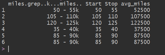
With that, we now have the complete cleaned data set. Since the code was run once for used car data and a second time for new car data, we have a total of 6000 observations equally divided between new and used. The final dimensions of the finished dataframe is 6000 observations of 12 variables, two of which are the description of the post and the link.

And now we have reached the visual aspect of the exploration. I want to see which model appears to have the most posts in this sample of ours. I’ve never used a mosaic plot before, but i guess there is always a first time.:

 
vcd::mosaic(~ Model + Car.Type, data = compiled_fac, 
            direction = c("v", "h"), highlighting="Car.Type", 
            highlighting_fill=c("light blue", "dark grey"), spacing = j)

I had to set the spacing to “2” because the labels for the Kancil, Kelisa, Kembara, and Kenari were overlapping each other. I couldn’t do much for the Nautica and Rusa. I’m not even sure if it’s possible to tilt the labels at an angle, like in ggplot2.

In any case, unsurprisingly, the ever-so prominent Myvi appears to be the most popular of Perodua’s cars; with the posts for used car sales being as much as the new ones. Following in popularity are the Viva and Alza, but there appear to be more New Car sales for the Viva  than Used Cars. There are only used car posts for the Kancil, Kelisa, Kembara, and Kenari. I would have been surprised if there were any new car posts for any of those, to be honest.

It seems that 2010 represents the biggest category of used cars, as far the model year is concerned, followed by the 2011 and 2012. I’m guessing it’s because people think they can perhaps get some kind of upgrade on their current cars by dishing the old ones and get a new one…Perodua or otherwise. The graph depicting this is below:

simple_sum = filter(compiled_fac, Car.Type == "UsedCar")
simple_sum = summarise(group_by(simple_sum, Year, Model), Count = length(Model))

ggplot(simple_sum, aes(reorder(Year,-Count), Count, fill = Model)) + 
  geom_bar(stat = "identity") +   #coord_flip() + 
  scale_fill_brewer(palette = "Paired") + 
  xlab("Model Year") + ggtitle("Number of sale posts, by Model and Year") + 
  theme(plot.title=element_text(size=16, face = "bold", color = "Black")) + 
  theme(axis.text.y=element_text(face = "bold", color = "black", size = 12), 
        axis.text.x=element_text(face = "bold", color = "black", size = 12))

I could go on about which groups represent what percentage of the data, but i reeeally want to start putting up some boxplots on the prices. But before i can do that, i had to manipulate the Engine.Cap variable so that there are only 6 categories: 0.66, 0.85, 1.00, 1.3, 1.5, and the 1.6. I haven’t added the code for this manipulations, but it’s nothing new. It’s just a matter of assigning the Engine.Cap column to a vector, removing all the “cc” using the str_replace_all() in the stringr package, changing all the 1500 to 1.5, 1295 to 1.3..and so on; and then assigning that vector back to the Engine.Cap column.

Now, on to the boxplots. Let’s take a look at a simple one of the car models VS the prices.

#No Mileage for new cars, remove column
simple_sum = select(compiled_fac, -Mileage)

simple_sum = filter(simple_sum, Car.Type == "NewCar")

simple_sum = na.omit(simple_sum)

x = seq(20000, 70000, by = 2000)

ggplot(simple_sum, aes(reorder(Model,-Price), Price)) + geom_boxplot(fill = "light blue") + 
  stat_summary(fun.y = "mean", geom="point", shape = 22, size = 2, fill = "red") + 
  scale_y_continuous(breaks = x) + 
  xlab("Model") + ggtitle("Boxplot: Car Model VS Price") + 
  theme(plot.title=element_text(size=16, face = "bold", color = "Black")) + 
  theme(axis.text.y=element_text(face = "bold", color = "black"), 
        axis.text.x=element_text(face = "bold", color = "black", size = 12))

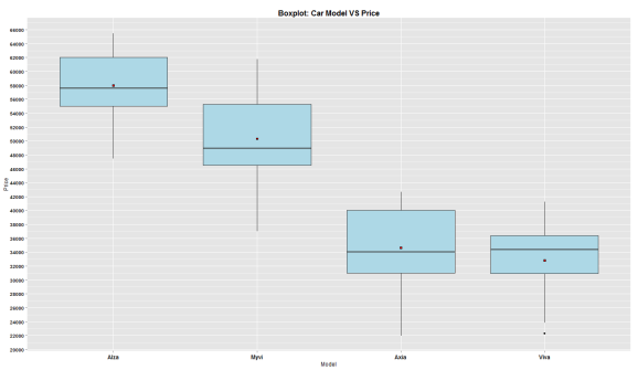
No big revelations here, but since the model is not the only factor that determines the price of a new car, i would like to see how the price differences look like when i add the transmission type

ggplot(simple_sum, aes(reorder(Model,-Price), Price)) + geom_boxplot(fill = "orange") + 
  stat_summary(fun.y = "mean", geom="point", shape = 22, size = 2, fill = "red") + 
  facet_grid(~Transm) + scale_y_continuous(breaks = x) + 
  xlab("Model") + ggtitle("Boxplot: Car Model VS Price, by Transmission Type") + 
  theme(plot.title=element_text(size=16, face = "bold", color = "Black")) + 
  theme(axis.text.y=element_text(face = "bold", color = "black"), 
        axis.text.x=element_text(face = "bold", color = "black", size = 12))

There seems to be a slight difference in prices for the Alza, Myvi, and Viva. The Axia, however, indicates a pretty big price difference if i was to judge solely on the transmission. But what about the engine capacity? I’m sure that must have some effect on how much the car would cost.

simple_sum = filter(simple_sum, Engine.Cap != 0.66, Engine.Cap != 0.85)

ggplot(simple_sum, aes(reorder(Model,Price), Price)) + geom_boxplot(fill = "light pink") + 
  stat_summary(fun.y = "mean", geom="point", shape = 22, size = 2, fill = "red") + 
  facet_grid(Transm~Engine.Cap) + scale_y_continuous(breaks = x) + 
  xlab("Model") + ggtitle("Boxplot: Car Model VS Price, by Transmission Type and Engine Capacity") + 
  theme(plot.title=element_text(size=16, face = "bold", color = "Black")) + 
  theme(axis.text.y=element_text(face = "bold", color = "black"), 
        axis.text.x=element_text(face = "bold", color = "black", size = 12))

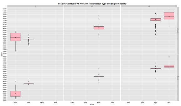
The only model affected by the engine capacity variable appears to be the Myvi, since you can get it in the 1.3 or the 1.5; there is a very apparent price difference between those two categories. However, selecting between transmissions shouldn’t be too much of a concern, considering the relatively small price difference. The same can’t be said for the Axia because of the very clear shift between the averages  when comparing prices according to transmission.

There is one more variable that is available in the dataset that would likely shed some more light on the price difference, and that is the model year.

 


ggplot(simple_sum, aes(reorder(Model,Price), Price, fill = Year)) + geom_boxplot() + 
  stat_summary(fun.y = "mean", geom="point", shape = 22, size = 2, fill = "red") + 
  facet_grid(Transm~Engine.Cap) + scale_y_continuous(breaks = x) + 
  xlab("Model") + ggtitle("Boxplot: Car Model VS Price, by Transmission Type, Engine Capacity, and Model Year") + 
  theme(plot.title=element_text(size=16, face = "bold", color = "Black")) + 
  theme(axis.text.y=element_text(face = "bold", color = "black"), 
        axis.text.x=element_text(face = "bold", color = "black", size = 12)) #+ scale_color_brewer(palette = "Dark2")

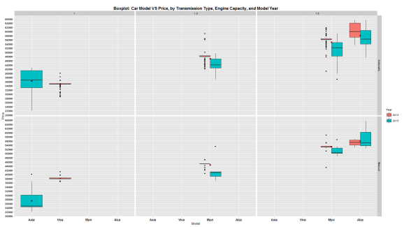
It would appear that the price difference between a 2014 and 2015 1.5L Alza on a manual transmission, is somewhat lower compared to an automatic with the same details. However there are noticeable difference in the case of the Myvi.

Last but not least, to satisfy my own curiosity, i was interested to see how the plot looked like isolating only for Myvis of the 2014 and 2015 variety:

simple_sum = select(compiled_fac, -Mileage)
simple_sum = filter(simple_sum, Model == "Myvi", Year == c("2015", "2014"))
simple_sum = na.omit(simple_sum)

x = seq(20000, 70000, by = 2000)

ggplot(simple_sum, aes(reorder(Model,Price), Price, fill = Year, color = Car.Type)) + geom_boxplot() + 
  stat_summary(fun.y = "mean", geom="point", shape = 22, size = 2, fill = "red") + 
  facet_wrap(Engine.Cap~Transm, nrow = 2) + scale_y_continuous(breaks = x) + 
  xlab("Model") + ggtitle("Comparing Used VS New Myvi - 1.3L VS 1.5L, 2014 VS 2015, and Manual VS Auto") + 
  theme(plot.title=element_text(size=16, face = "bold", color = "Black")) + 
  theme(axis.text.y=element_text(face = "bold", color = "black"), 
        axis.text.x=element_text(face = "bold", color = "black", size = 12)) + 
  scale_fill_brewer(palette = "Dark2") + scale_color_brewer(palette = "Set1")

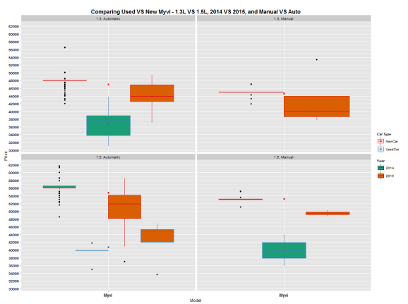
I expected a pretty big price difference between a new 2014 and a used 2014, but i figured the new and used 2015 would not have  a gap that is as noticeable

It’s possible to explore and visualize the data in other ways, and likely in ways that are better than mine – since i’m only starting out. It’s maybe even possible to develop a model to determine the price of a used car using the data  – but i’m not exactly certain how to go about that. I would need to at least finish the regression models course on coursera for me to be certain of that i’m doing.

As always, the data file is below and you can play around with it as much as you’d like.

Final_CarList_Compiled.csv