
Seeing India through Food – An Experiment in Multidimensional Scaling
Want to share your content on R-bloggers? click here if you have a blog, or here if you don't.
The ‘Household Consumption of Various Goods and Services in India’ report from the National Sample Survey Office (NSSO), Government of India includes survey data on the monthly per capita quantity of consumption of selected food items. The report is available from http://mospi.nic.in/Mospi_New/Admin/publication.aspx (a registration is required). The per capita quantity of consumption data is provided for every state and union territory of India, separately for rural and urban sectors. Here is a snapshot of the data for the urban sector from the February 2012 report:
| rice.kg | wheat.kg | arhar.kg | moong.kg | masur.kg | urd.kg | … | |
| AndhraPradesh | 8.764 | 0.656 | 0.412 | 0.095 | 0.032 | 0.173 | |
| ArunachalPradesh | 10.49 | 0.763 | 0.066 | 0.079 | 0.296 | 0.007 | |
| Assam | 10.246 | 1.109 | 0.044 | 0.105 | 0.363 | 0.047 | |
| Bihar | 5.804 | 5.732 | 0.088 | 0.057 | 0.222 | 0.025 | |
| Chhattisgarh | 7.643 | 2.686 | 0.685 | 0.024 | 0.053 | 0.054 | |
| … |
The results of an analysis of this food consumption data using Multidimensional Scaling (MDS) is presented in this post. The objective behind this analysis was to see what kind of clustering patterns are seen among the states of India, as far as food consumption goes.
MDS was carried out using R (version 3.1.2) using the isoMDS() function from the MASS package and using the ‘manhattan’ distance measure. The plot below is a visualization of the results from the MDS (only for the sake of clarity, the union territories are not shown in the plot):
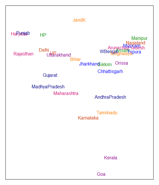
Here is a map of India to compare the above plot with. Don’t you think that the relative positioning of the different states in India nicely captured in the MDS analysis?
It is often said that the culinary diversity in India is the result of the diversity in the geography, climate, economy, tradition and culture within the country. All of these factors also contribute to an extent on the consumption of basic food items, resulting in the clustering together of geographically and culturally nearby regions even though the data analyzed was on food.
Some more ‘food’ for thought:
- Though Goa is geographically close to the states of Karnataka and Maharashtra, with respect to the food consumption pattern, Goa seems closer to Kerala. This is probably reflecting the strong coastal influence for both Goa and Kerala. Karnataka and Maharashtra too have a long coastline, but the influence of the inland may have diminished the coastal effects. In contrast, Kerala being narrow, the influence of the sea is strong in its cuisine. The relative positioning of Sikkim too, is a bit off. Not able to understand the reason for this.
- What would a MDS plot using data from rural areas alone or from urban areas alone look like? This would be a topic for a future post.
- The NSSO has meanwhile made available a more recent report in 2014. We can explore how the data from the newer report compares to the 2012 data.

R-bloggers.com offers daily e-mail updates about R news and tutorials about learning R and many other topics. Click here if you're looking to post or find an R/data-science job.
Want to share your content on R-bloggers? click here if you have a blog, or here if you don't.