Periodic matrix model for annual plant demography
Want to share your content on R-bloggers? click here if you have a blog, or here if you don't.
Let’s challenge to build a matrix population model of annual organisms and then calculate the population growth rate λ using R.
Consider a simple life cycle of imaginary annual plants; that germinate in spring, flower in summer, produce seeds in autumn, and are dead in winter. Though parent plants are dead in winter, dormant seeds are alive in soil. Some of the seeds germinate in subsequent spring; others continue to be dormant.
The first thing to do is to build a stage-classified life cycle graph. The second is to define transition matrices that describe the graph. At last, solving the characteristic equation of the matrices gives a stable population growth rate, namely, λ.
1. Life cycle graph
Seasonal stages of life of such an annual plant are shown below.
| Season | Stages |
|---|---|
| Spring | seedlings, seeds |
| Summer | flowering plants, seeds |
| Autumn | seed production stages, seeds |
| Winter | seeds |
A four seasonal life cycle graph is as below (Fig. 1).
2. Matrix
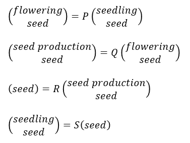
The life cycle graph of Fig. 1 is represented by four transition matrices (P, Q, R and S) and population structure vectors. The matrix P represents a transition from spring to summer. Q is from summer to autumn; R is from autumn to winter; and S is from winter to spring.
I chose four important components to describe the life cycle graph.
seed  <- 0.9^4  # Seed surviving rate; annual
germ  <- 0.3    # Germination rate; spring
plant <- 0.05   # Plant surviving rate; from germination to mature
yield <- 100    # Seed production number; per matured plant
Additionally, pollination rate of flower (or maturing rate) was used to divide the plant surviving rate before and after flowering.
mature <- 0.5 # pollination rate
I defined here all scripts using 'function()'; functions without arguments.
For example, I wrote 'seedq <- function() seed^(1/4)', not 'seedq <- seed^(1/4)' nor 'seedq <- function(seed) seed^(1/4)'.
This was because I wanted them to be recalculated automatically when I changed the values of 5 parameters chosen above. And also I decided to make the parameters global for simplicity. This idea works for tiny scripts, but will not for a larger one. Guys loving principles of scripting, or using delicate functions such as 'apply’, may change these scripts not to use global variables.
seedq             <- function() seed^(1/4)
# assume constant seed surviving rate through all seasons.

p11               <- function() plant / mature
q11               <- function() mature
r11               <- function() yield
s11               <- function() germ * seedq()
s21               <- function() (1 - germ) * seedq()
p22 <- q22 <- r12 <- function() seedq()
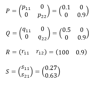
Then transition matrices of four seasons will be as follows (Fig. 3).
P <- function() matrix(data=c(
          p11(), 0    ,
          0    , p22()
        ), nrow=2, ncol=2, byrow=T)

Q <- function() matrix(data=c(
          q11(), 0    ,
          0    , q22()
        ), nrow=2, ncol=2, byrow=T)

R <- function() matrix(data=c(
          r11(), r12()
        ), nrow=1, ncol=2, byrow=T)

S <- function() matrix(data=c(
          s11(),
          s21()
        ), nrow=2, ncol=1, byrow=T)
The population growth rate from year t to year t + 1 is represented by an annual transition matrix (Fig. 4).
For the annual plant above, there are four different annual cycles based on four start seasons (Fig. 5).
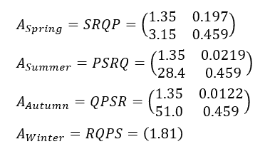
Annual transition matrices are calculated by products of these seasonal matrices (Fig. 6).
A.spring <- function() S() %*% R() %*% Q() %*% P()
A.summer <- function() P() %*% S() %*% R() %*% Q()
A.autumn <- function() Q() %*% P() %*% S() %*% R()
A.winter <- function() R() %*% Q() %*% P() %*% S()
Annual matrix starting at winter is 1×1, namely, a scalar 1.81.
3. Population growth rate
Because no parent plants survive winter, the winter population consists of seed only. So this scalar is exactly the value of population growth λ (Fig. 7).
Every annual matrix A gives same λ regardless of start season, because the annual growing rate of the population must be consistent. Let’s check it.
For 2×2 matrix A (Spring, Summer and Autumn), a stable growth rate is a solution of the characteristic equation below (Fig. 8).
The λ, the stable growth rate, is the dominant eigenvalue. The w, the stable population structure, is the eigenvector corresponding to the λ.
lambda <- function(A) eigen(A)$values[1]
# output of eigenvalues is decreasingly sorted.

lambda(A.spring())
lambda(A.summer())
lambda(A.autumn())
lambda(A.winter())
The results are λ = 1.81 for all four cases.
Fortunately, R can handle more complex matrices than 2×2. This simple procedure will work for complex life cycles that have more than two stages or additional paths.
References
- Caswell, H., 2001. Matrix Population Models: Construction, Analysis, and Interpretation, Sinauer Associates.
ISBN 9780878930968
R-bloggers.com offers daily e-mail updates about R news and tutorials about learning R and many other topics. Click here if you're looking to post or find an R/data-science job.
Want to share your content on R-bloggers? click here if you have a blog, or here if you don't.


