Following yesterday’s post on Rao’s, Liu’s, and Dunson’s paper on a new approach to intractable normalising constants, and taking advantage of being in Warwick, I tested the method on a toy model, namely the posterior associated with n Student’s t observations with unknown location parameter μ and a flat prior,

which is “naturally” bounded by a Cauchy density with scale √ν. The constant M is then easily derived and running the new algorithm follows from a normal random walk proposal targeting the augmented likelihood (R code below).

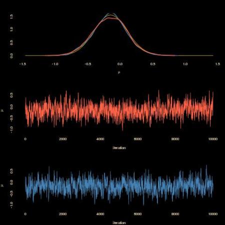
As shown by the above graph, the completion-by-rejection scheme produces a similar outcome (tomato) as the one based on the sole observations (steelblue). With a similar acceptance rate. However, the computing time is much much degraded:

> system.time(g8())
   user  system elapsed
 53.751   0.056  54.103
> system.time(g9())
   user  system elapsed
  1.156   0.000   1.161

when compared with the no-completion version. Here is the entire R code that produced both MCMC samples:

#Student t observations and flat prior
nu=4
n=25
M=pi*sqrt(nu)
sqrtnu=sqrt(nu)
obs=rt(n,df=4)
sdobs=sd(obs)

#unormalised t
mydt=function(x,mu){
  return(dt(x-mu,df=nu)/dt(0,df=nu))}
mydtc=cmpfun(mydt)

mydcauchy=function(x,mu){
  y=(x-mu)/sqrtnu
  return(dcauchy(y)/sqrtnu)}
mydcaucchy=cmpfun(mydcauchy)

#augmented data
augmen=function(mu){
y=NULL
for (i in 1:n){
  prop=mu+rcauchy(1)*sqrtnu
  reject=(runif(1)<mydtc(prop,mu)/(M*mydcaucchy(prop,mu)))
  while (!reject){
    y=c(y,prop)
    prop=mu+rcauchy(1)*sqrtnu
    reject=(runif(1)<mydtc(prop,mu)/(M*mydcaucchy(prop,mu)))}
  }
return(y)}

#Gibbs
gibbsda=function(T=10^4){
theta=rep(0,T)
for (t in 2:T){
   rej=augmen(theta[t-1])
   theta[t]=prop=theta[t-1]+rnorm(1,sd=.1*sdobs)
   propdens=sum(dt(obs-prop,df=nu,log=TRUE))+
     sum(log(mydcaucchy(rej,prop)-mydtc(rej,mu=prop)/M))
   refdens=sum(dt(obs-theta[t-1],df=nu,log=TRUE))+
     sum(log(mydcaucchy(rej,theta[t-1])-mydtc(rej,mu=theta[t-1])/M))
   if (log(runif(1))>propdens-refdens) theta[t]=theta[t-1]
   }
return(theta)}
g8=cmpfun(gibbsda)

gibbs2=function(T=10^4){
eta=rep(0,T)
for (t in 2:T){
   eta[t]=prop=eta[t-1]+rnorm(1,sd=sdobs)
   propdens=sum(dt(obs-prop,df=nu,log=TRUE))
   refdens=sum(dt(obs-eta[t-1],df=nu,log=TRUE))
   if (log(runif(1))>propdens-refdens) eta[t]=eta[t-1]
   }
return(eta)}
g9=cmpfun(gibbsda)