
Pimping your forest plot
Want to share your content on R-bloggers? click here if you have a blog, or here if you don't.

In order to celebrate my Gmisc-package being on CRAN I decided to pimp up the forestplot2 function. I had a post on this subject and one of the suggestions I got from the comments was the ability to change the default box marker to something else. This idea had been in my mind for a while and I therefore put it into practice.
Forest plots (sometimes concatenated into forestplot) date back at least to the wild ’70s. They are an excellent tool to display lots of estimates and confidence intervals. Traditionally they’ve been used in meta-analyses although I think the use is spreading and I’ve used them a lot in my own research.
For convenience I’ll use the same setup in the demo as in the previous post:
1 2 3 4 5 6 7 8 9 10 11 12 13 14 15 16 17 18 19 20 21 22 23 24 25 26 | library(Gmisc)
Sweden <-
structure(
c(0.0408855062954068, -0.0551574080806885,
-0.0383305964199184, -0.0924757229652802,
0.0348395599810297, -0.0650808763059716,
-0.0472794647337126, -0.120200006386798,
0.046931452609784, -0.0452339398554054,
-0.0293817281061242, -0.0647514395437626),
.Dim = c(4L, 3L),
.Dimnames = list(c("Males vs Female", "85 vs 65 years",
"Charlsons Medium vs Low", "Charlsons High vs Low"),
c("coef", "lower", "upper")))
Denmark <-
structure(
c(0.0346284183072541, -0.0368279085760325,
-0.0433553672510346, -0.0685734649940999,
0.00349437418972517, -0.0833673052667752,
-0.0903366633240568, -0.280756832078775,
0.065762462424783, 0.00971148811471034,
0.00362592882198759, 0.143609902090575),
.Dim = c(4L, 3L),
.Dimnames = list(c("Males vs Female", "85 vs 65 years",
"Charlsons Medium vs Low", "Charlsons High vs Low"),
c("coef", "lower", "upper"))) |
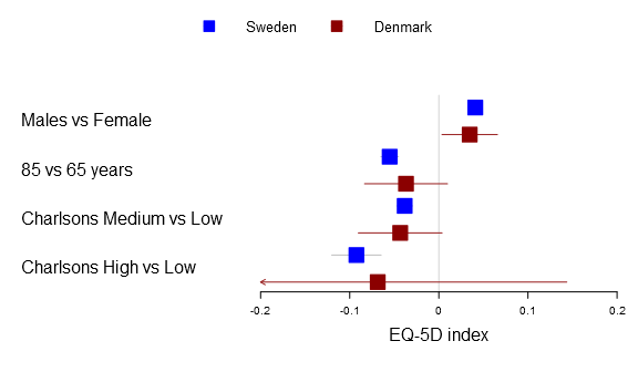
Here is the basic multi-line forest plot:
1 2 3 4 5 6 7 8 9 10 11 12 13 14 15 16 | forestplot2(mean=cbind(Sweden[,"coef"], Denmark[,"coef"]),
lower=cbind(Sweden[,"lower"], Denmark[,"lower"]),
upper=cbind(Sweden[,"upper"], Denmark[,"upper"]),
labeltext=rownames(Sweden),
legend=c("Sweden", "Denmark"),
# Added the clip argument as some of
# the Danish CI are way out therer
clip=c(-.2, .2),
# Getting the ticks auto-generate is
# a nightmare - it is usually better to
# specify them on your own
xticks=c(-.2, -.1, .0, .1, .2),
boxsize=0.3,
col=fpColors(box=c("blue", "darkred")),
xlab="EQ-5D index",
new_page=TRUE) |
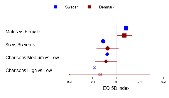
The package comes with the following functions for drawing each confidence interval:
- fpDrawNormalCI – the regular box confidence interval
- fpDrawCircleCI – draws a circle instead of a box
- fpDrawDiamondCI – draws a diamond instead of a box
- fpDrawPointCI – draws a point instead of a box
- fpDrawSummaryCI – draws a summary diamond
Below you can find the all four alternatives:
1 2 3 4 5 6 7 8 9 10 11 12 13 14 15 16 17 18 | forestplot2(mean=cbind(Sweden[,"coef"], Denmark[,"coef"]),
lower=cbind(Sweden[,"lower"], Denmark[,"lower"]),
upper=cbind(Sweden[,"upper"], Denmark[,"upper"]),
labeltext=rownames(Sweden),
legend=c("Sweden", "Denmark"),
clip=c(-.2, .2),
xticks=c(-.2, -.1, .0, .1, .2),
boxsize=0.3,
col=fpColors(box=c("blue", "darkred")),
# Set the different functions
confintNormalFn=
list(fpDrawNormalCI,
fpDrawCircleCI,
fpDrawDiamondCI,
fpDrawPointCI),
pch=13,
xlab="EQ-5D index",
new_page=TRUE) |
The confintNormalFn accepts either a single function, a list of functions, a function name, or a vector/matrix of names. If the list is one-leveled or you have a vector in a multi-line situation it will try to identify if the length matches row or column. The function tries to rewrite to match your the dimension of your multi-line plot, hence you can write:
1 2 3 4 5 6 7 8 9 10 11 12 13 14 15 16 17 18 | # Changes all to diamonds
confintNormalFn="fpDrawDiamondCI"
# The Danish estimates will appear as a circle while
# Swedes will be as a diamond
confintNormalFn=list(fpDrawDiamondCI, fpDrawCircleCI)
# Changes first and third row to diamond + circle
confintNormalFn=list(list(fpDrawDiamondCI, fpDrawCircleCI),
list(fpDrawNormalCI, fpDrawNormalCI),
list(fpDrawDiamondCI, fpDrawCircleCI),
list(fpDrawNormalCI, fpDrawNormalCI))
# The same as above but as a matrix diamond + circle
confintNormalFn=rbind(c("fpDrawDiamondCI", "fpDrawCircleCI"),
c("fpDrawNormalCI", "fpDrawNormalCI"),
c("fpDrawDiamondCI", "fpDrawCircleCI"),
c("fpDrawNormalCI", "fpDrawNormalCI")) |
If you use the same number of lines as the lines the legend will automatically use your custom markers although you can always just use the legendMarkerFn argument:
1 2 3 4 5 6 7 8 9 10 11 12 13 14 15 16 | forestplot2(mean=cbind(Sweden[,"coef"], Denmark[,"coef"]),
lower=cbind(Sweden[,"lower"], Denmark[,"lower"]),
upper=cbind(Sweden[,"upper"], Denmark[,"upper"]),
labeltext=rownames(Sweden),
legend=c("Sweden", "Denmark"),
legend.pos=list(x=0.8,y=.4),
legend.gp = gpar(col="#AAAAAA"),
legend.r=unit(.1, "snpc"),
clip=c(-.2, .2),
xticks=c(-.2, -.1, .0, .1, .2),
boxsize=0.3,
col=fpColors(box=c("blue", "darkred")),
# Set the different functions
confintNormalFn=c("fpDrawDiamondCI", "fpDrawCircleCI"),
xlab="EQ-5D index",
new_page=TRUE) |
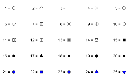
Now for the pch-argument in the fpDrawPointCI you can use any of the predefined integers:
1 2 3 4 5 6 7 8 9 10 11 12 13 | grid.newpage()
for(i in 1:5){
grid.text(sprintf("%d = ", ((i-1)*5+1:5)),
just="right",
x=unit(seq(.1, .9, length.out=5), "npc")-unit(3, "mm"),
y=unit(rep(seq(.9, .1, length.out=5)[i], times=5), "npc"))
grid.points(x=unit(seq(.1, .9, length.out=5), "npc"),
y=unit(rep(seq(.9, .1, length.out=5)[i], times=5), "npc"),
pch=((i-1)*5+1:5),
gp=gpar(col="black", fill="blue"))
} |
If you are still not satisfied you have always the option of writing your own function. I suggest you start with copying the fpDrawNormalCI and see what you want to change:
1 2 3 4 5 6 7 8 9 10 11 12 13 14 15 16 17 18 19 20 21 22 23 24 25 26 27 28 29 30 31 32 33 34 35 36 37 38 39 40 41 42 43 44 45 46 47 48 49 50 51 52 53 54 55 56 57 58 59 60 61 62 63 64 65 66 67 68 69 | fpDrawNormalCI <- function(lower_limit,
estimate,
upper_limit,
size,
y.offset = 0.5,
clr.line, clr.marker,
lwd,
...) {
# Draw the lines if the lower limit is
# actually below the upper limit
if (lower_limit < upper_limit){
# If the limit is outside the 0-1 range in npc-units
# then that part is outside the box and it should
# be clipped (this function adds an arrow to the end
# of the line)
clipupper <-
convertX(unit(upper_limit, "native"),
"npc",
valueOnly = TRUE) > 1
cliplower <-
convertX(unit(lower_limit, "native"),
"npc",
valueOnly = TRUE) < 0
if (clipupper || cliplower) {
# A version where arrows are added to the part outside
# the limits of the graph
ends <- "both"
lims <- unit(c(0, 1), c("npc", "npc"))
if (!clipupper) {
ends <- "first"
lims <- unit(c(0, upper_limit), c("npc", "native"))
}
if (!cliplower) {
ends <- "last"
lims <- unit(c(lower_limit, 1), c("native", "npc"))
}
grid.lines(x = lims,
y = y.offset,
arrow = arrow(ends = ends,
length = unit(0.05, "inches")),
gp = gpar(col = clr.line, lwd=lwd))
} else {
# Don't draw the line if it's no line to draw
grid.lines(x = unit(c(lower_limit, upper_limit), "native"), y = y.offset,
gp = gpar(col = clr.line, lwd=lwd))
}
}
# If the box is outside the plot the it shouldn't be plotted
box <- convertX(unit(estimate, "native"), "npc", valueOnly = TRUE)
skipbox <- box < 0 || box > 1
# Lastly draw the box if it is still there
if (!skipbox){
# Convert size into 'snpc'
if(!is.unit(size)){
size <- unit(size, "snpc")
}
# Draw the actual box
grid.rect(x = unit(estimate, "native"),
y = y.offset,
width = size,
height = size,
gp = gpar(fill = clr.marker,
col = clr.marker))
}
} |
The estimate and the confidence interval points are provided as raw numbers and are assumed to be “native”, that is their value is the actual coefficient and is mapped correctly as is.
Note that all the regression functions in the Gmisc-package have moved to the Greg-package, soon to be available on CRAN… but until I have added some more unit tests you need to use the GitHub version.
![]()
R-bloggers.com offers daily e-mail updates about R news and tutorials about learning R and many other topics. Click here if you're looking to post or find an R/data-science job.
Want to share your content on R-bloggers? click here if you have a blog, or here if you don't.