
The forestplot of dreams
Want to share your content on R-bloggers? click here if you have a blog, or here if you don't.

Displaying large regression models without overwhelming the reader can be challenging. I believe that forestplots are amazingly well suited for this. The plot gives a quick understanding of the estimates position in comparison to other estimates, while also showcasing the uncertainty. This project started with some minor tweaks to prof. Thomas Lumleys forestplot and ended up in a complete remake of the function. In this post I’ll show you how to tame the plot using data from my latest article.
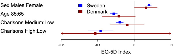
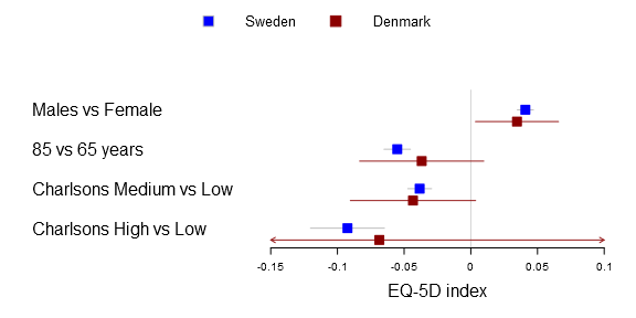
I’ve used the plots in my two latest publications and they have had a warm reception. In the latest study we compared Swedish with Danish patient’s health related quality of life after a total hip arthroplasty. We were interested in comparing if there was a difference between common explanatory variables in Denmark and Sweden, i.e. the generalizability. The Swedish data set was vast while the Danish was a tiny sample resulting in very different confidence intervals. You can find the main graph below.
Gordon et al. BMC Musculoskeletal Disorders 2013 14:316 doi:10.1186/1471-2474-14-316
Tutorial data
Below you can find a data dump for the estimates that I used to generate the plot.
1 2 3 4 5 6 7 8 9 10 11 12 13 14 15 16 17 18 19 20 21 | Sweden <-
structure(
c(0.0408855062954068, -0.0551574080806885, -0.0383305964199184,
-0.0924757229652802, 0.0348395599810297, -0.0650808763059716,
-0.0472794647337126, -0.120200006386798, 0.046931452609784,
-0.0452339398554054, -0.0293817281061242, -0.0647514395437626),
.Dim = c(4L, 3L),
.Dimnames = list(c("Males vs Female", "85 vs 65 years",
"Charlsons Medium vs Low", "Charlsons High vs Low"),
c("coef", "lower", "upper")))
Denmark <-
structure(
c(0.0346284183072541, -0.0368279085760325, -0.0433553672510346,
-0.0685734649940999, 0.00349437418972517, -0.0833673052667752,
-0.0903366633240568, -0.280756832078775, 0.065762462424783,
0.00971148811471034, 0.00362592882198759, 0.143609902090575),
.Dim = c(4L, 3L),
.Dimnames = list(c("Males vs Female", "85 vs 65 years",
"Charlsons Medium vs Low", "Charlsons High vs Low"),
c("coef", "lower", "upper"))) |
The forestplot tutorial
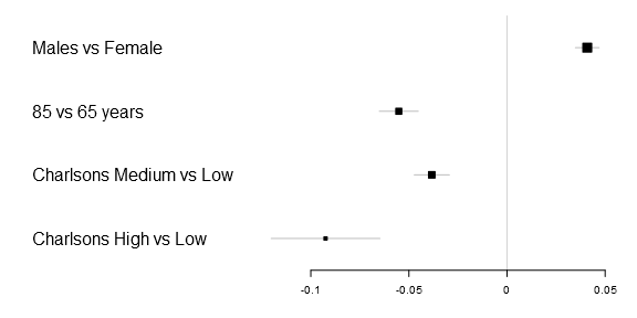
Lets start with the basic code to generate a simple forestplot. The xticks parameter is not necessary but in this particular example the 0.05 tick is otherwise not included and I therefore added it. Note: you need to download my package, you can find the Gmisc-package here, for this tutorial to work.
1 2 3 4 5 6 | library(Gmisc)
forestplot2(mean=Sweden[,"coef"],
lower=Sweden[,"lower"],
upper=Sweden[,"upper"],
labeltext=rownames(Sweden),
xticks=c(-.1, -.05, 0, .05)) |
Greek letters
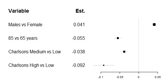
One of the first things that got me tweaking the original forestplot function was that I wanted to have a simple expression in the header. Getting a matrix into the original function was rather simple, as you can see below:
1 2 3 4 5 6 7 8 9 10 11 12 13 14 15 16 17 18 19 | # Prepare a new matrix where the top row is empty
Sweden_w_header <- rbind(rep(NA,times=ncol(Sweden)),
Sweden)
# Add a row name
rownames(Sweden_w_header)[1] <- "Variable"
# Create the matrix
lab_mtrx <- cbind(rownames(Sweden_w_header),
append("Est.",
round(Sweden_w_header[,"coef"],3)[2:5]))
# Do the actual plot
forestplot2(mean=Sweden_w_header[,"coef"],
lower=Sweden_w_header[,"lower"],
upper=Sweden_w_header[,"upper"],
labeltext=lab_mtrx,
is.summary=c(TRUE, rep(FALSE, times=nrow(Sweden_w_header)-1)),
xticks=c(-.1, -.05, 0, .05),
new_page=TRUE) |
As many of you know it is impossible to combine different types in one matrix/vector and you therefore need to supple the function a list. The number of elements in the list have to be m x n as in any matrix, below is the example plot that I was originally aiming for:
1 2 3 4 5 6 7 8 9 10 11 12 13 | # Generate a labellist
lab_list <- list(rownames(Sweden_w_header),
append(list(expression(beta)),
round(Sweden_w_header[,"coef"],3)[2:5]))
# Do the actual plot
forestplot2(mean=Sweden_w_header[,"coef"],
lower=Sweden_w_header[,"lower"],
upper=Sweden_w_header[,"upper"],
labeltext=lab_list,
is.summary=c(TRUE, rep(FALSE, times=nrow(Sweden_w_header)-1)),
xticks=c(-.1, -.05, 0, .05),
new_page=TRUE) |
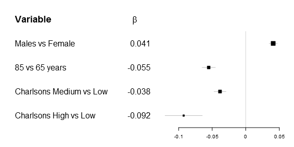
Ironically after figuring this out my main supervisor correctly pointed out, while the β is correct – it doesn’t really add that much while there is a risk of alienating less statistically oriented readers…
Multi-line forestplots
After this set-back I was at least familiar with the forestplot function allowing further tweaking. Early on I realized that it can be convenient to display the same risk factors multiple times. The idea was that in situations where there are different outcomes, for instance hip replacement re-operation due to infection, dislocation or fracture it can be useful to see the estimates adjacent to each-other. I also used it for comparing Cox proportional hazards models with competing risk regressions and Poisson regression. It turned out to be rather useful.
In the Sweden/Denmark paper the comparison is simply between countries. The code is fairly straight forward, you now need to have to provide the function with a m x n matrix for the mean, lower and upper parameters. The n should be the number of comparison groups, in the Sweden vs Denmark paper the groups are two:
1 2 3 4 5 6 7 8 9 10 11 12 13 | forestplot2(mean=cbind(Denmark[,"coef"], Sweden[,"coef"]),
lower=cbind(Denmark[,"lower"], Sweden[,"lower"]),
upper=cbind(Denmark[,"upper"], Sweden[,"upper"]),
labeltext=rownames(Sweden),
legend=c("Denmark", "Sweden"),
# Added the clip argument as some of
# the Danish CI are way out therer
clip=c(-.15, .1),
boxsize=0.3,
col=fpColors(box=c("darkred", "blue"),
line=c("darkred", "blue")),
xlab="EQ-5D index",
new_page=TRUE) |
Originally I was using the legend() function but it turned out to be rather complicated. You can now achieve the same things with the legend parameters, here’s an example with a rounded box at the top left corner:
1 2 3 4 5 6 7 8 9 10 11 12 13 14 15 16 | forestplot2(mean=cbind(Denmark[,"coef"], Sweden[,"coef"]),
lower=cbind(Denmark[,"lower"], Sweden[,"lower"]),
upper=cbind(Denmark[,"upper"], Sweden[,"upper"]),
labeltext=rownames(Sweden),
legend=c("Denmark", "Sweden"),
legend.pos=list("topleft"),
legend.r=unit(.2, "npc"),
legend.gp=gpar(col="grey", fill="#FAFAFF"),
# Added the clip argument as some of
# the Danish CI are way out therer
clip=c(-.15, .1),
boxsize=0.3,
col=fpColors(box=c("darkred", "blue"),
line=c("darkred", "blue")),
xlab="EQ-5D index",
new_page=TRUE) |

I hope you’ll find the forestplot function as useful as I have.
![]()
R-bloggers.com offers daily e-mail updates about R news and tutorials about learning R and many other topics. Click here if you're looking to post or find an R/data-science job.
Want to share your content on R-bloggers? click here if you have a blog, or here if you don't.