I've finally had some success at munging some HTML. For quite some time, I've wanted to render a county level choropleth for US presidential election results. The numbers are all there on Politico.com, but attempts to use readHTMLTable never returned the full set of data. It still doesn't, but I have sorted out how to get all of the results I want. It takes a fair bit of work, but- once the smoke clears- doesn't seem too crazy.

First, we'll fetch some raw HTML for North Carolina.

library(XML)

URL = "http://www.politico.com/2012-election/results/president/north-carolina/"
content.raw = htmlParse(URL, useInternalNodes = TRUE)

Inspection of the tables which get returned tell us that the second element in the list has the data we need. Attempts to extract the information lead us to take a slightly different approach. First, we'll get all the nodes with a “tbody” element. Each of these nodes may be treated as a table.

tables <- getNodeSet(content.raw, "//table")
counties = getNodeSet(tables[[2]], "//tbody")
counties = counties[-1]

countyTables = lapply(counties, readHTMLTable, header = FALSE, stringsAsFactors = FALSE)

The table we get isn't quite what we want.

head(countyTables[[1]])

##                          V1        V2    V3     V4     V5
## 1 Alamance 100.0% Reporting M. Romney   GOP  56.6% 37,712
## 2              B. Obama (i)       Dem 42.5% 28,341   <NA>
## 3                G. Johnson       Lib  0.9%    585   <NA>

A couple helper functions will fetch the county name and move the cells to a sensible location.

GetCountyName = function(dfCounty) {
    strCounty = dfCounty[1, 1]
    strCounty = strsplit(strCounty, " ")
    strCounty[[1]][1]
}

MungeTable = function(dfCounty) {

    if (ncol(dfCounty) != 5) 
        return(data.frame())

    dfCounty[1, 1] = GetCountyName(dfCounty)

    dfCounty[-1, 2:5] = dfCounty[-1, 1:4]

    dfCounty[, 1] = dfCounty[1, 1]

    colnames(dfCounty) = c("CountyName", "Candidate", "Party", "Pct", "Votes")

    dfCounty$Votes = gsub(",", "", dfCounty$Votes)
    dfCounty$Votes = as.numeric(dfCounty$Votes)

    dfCounty$Pct = NULL

    dfCounty
}

correctTable = MungeTable(countyTables[[1]])
head(correctTable)

##   CountyName    Candidate Party Votes
## 1   Alamance    M. Romney   GOP 37712
## 2   Alamance B. Obama (i)   Dem 28341
## 3   Alamance   G. Johnson   Lib   585

With that done, it's a simple thing to munge each data frame and then bind the results into a single data frame.

counties = lapply(countyTables, MungeTable)
dfNorthCarolina = do.call("rbind", counties)

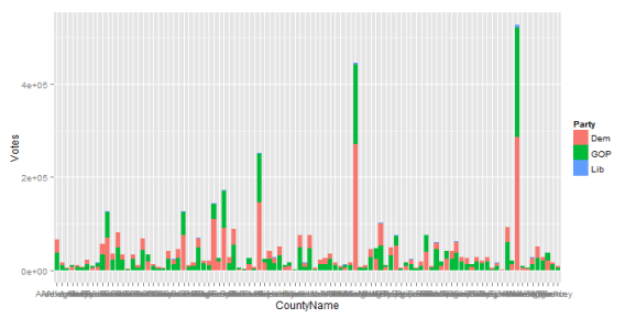
A plot shows that Obama won in counties with a high population, but didn't do as well in smaller counties. I'll draw some better charts tomorrow.

library(ggplot2)
ggplot(dfNorthCarolina, aes(x = CountyName, y = Votes, fill = Party)) + geom_bar(stat = "identity")

This required getting very, very familiar with the underlying HTML structure. That's a hassle, but hardly impossible. Tomorrow, this will become a map and I'll make some inferences about voting patterns and demographics.

sessionInfo()

## R version 3.0.2 (2013-09-25)
## Platform: x86_64-w64-mingw32/x64 (64-bit)
## 
## locale:
## [1] LC_COLLATE=English_United States.1252 
## [2] LC_CTYPE=English_United States.1252   
## [3] LC_MONETARY=English_United States.1252
## [4] LC_NUMERIC=C                          
## [5] LC_TIME=English_United States.1252    
## 
## attached base packages:
## [1] stats     graphics  grDevices utils     datasets  methods   base     
## 
## other attached packages:
## [1] XML_3.98-1.1     knitr_1.4.1      RWordPress_0.2-3 ggplot2_0.9.3.1 
## [5] reshape2_1.2.2   plyr_1.8        
## 
## loaded via a namespace (and not attached):
##  [1] colorspace_1.2-3   dichromat_2.0-0    digest_0.6.3      
##  [4] evaluate_0.4.7     formatR_0.9        grid_3.0.2        
##  [7] gtable_0.1.2       labeling_0.2       markdown_0.6.3    
## [10] MASS_7.3-29        munsell_0.4.2      proto_0.3-10      
## [13] RColorBrewer_1.0-5 RCurl_1.95-4.1     scales_0.2.3      
## [16] stringr_0.6.2      tools_3.0.2        XMLRPC_0.3-0