Earlier today, while looking for something else, I managed to stumble across a presentation given at the 2010 CAS RPM. (Egregious self-promotion: I'll be leading a day-long workshop at next year's RPM in Washington, DC.) I wasn't looking for a presentation on hierarchical models, but there one was. The fantastic Jim Guszcza has a great slide show on hierarchical models in an actuarial context. Actually, it's so great that you should stop reading this post now, go read Jim's presentation and prepare to spend the next few hours reading everything that Jim has written

Anyone still reading this? OK, so a few days ago, I simulated some Poisson claims. This is the first step of what will one day be a multi-level simulation. I'm doing this solely to get better at understanding how to fit multi-level/hierachical models. I tend to learn random process best by simulating them first. I'll confess that I was a bit disappointed by that first post. I think that stems largely from the fact that I had very few observations and that the “between” variance was so much larger than the “within” variance. That is to say that I had begun by presuming a “root” Poisson process for the entire United States and that each of the 51 states has its own Poisson. This is likely too simple a model. I'm going to forego additional layers of the model and- for now- augment the state level process by simulating a lot more claims. Each state will have 10,000 policies, each of which will have its own set of claims. If I can stay awake long enough, I'll try to add some state-level overdispersion and see what it does to the simulations and the fit. (Aside: I'm shifting from 51 to 50 states so that I can lazily add an abbreviation)

The first code chunk will be a repeat from Sunday's post. I'll execute it, but not display the code. At this stage, I have 51 lambdas that have been simulated from a gamma distribution with a scale of 14.0412 and a shape parameter of 0.7122. (Again, this code has been evaluated, but not echoed. That same code is may be seen here.)

library(datasets)
numPolicies = 10000
dfPolicies = as.data.frame(expand.grid(1:numStates, 1:numPolicies))
colnames(dfPolicies) = c("State", "PolicyID")
dfPolicies$Lambda = lambdas[dfPolicies$State]
dfPolicies$NumClaims = rpois(nrow(dfPolicies), dfPolicies$Lambda)
dfPolicies$Postal = state.abb[dfPolicies$State]

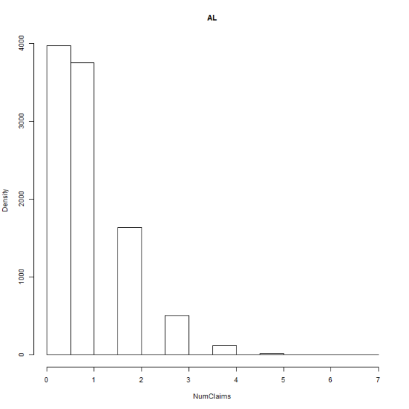
hist(dfPolicies$NumClaims[dfPolicies$State == 1], xlab = "NumClaims", ylab = "Density", 
    main = state.abb[1])

hist(dfPolicies$NumClaims[dfPolicies$State == 2], xlab = "NumClaims", ylab = "Density", 
    main = state.abb[2])

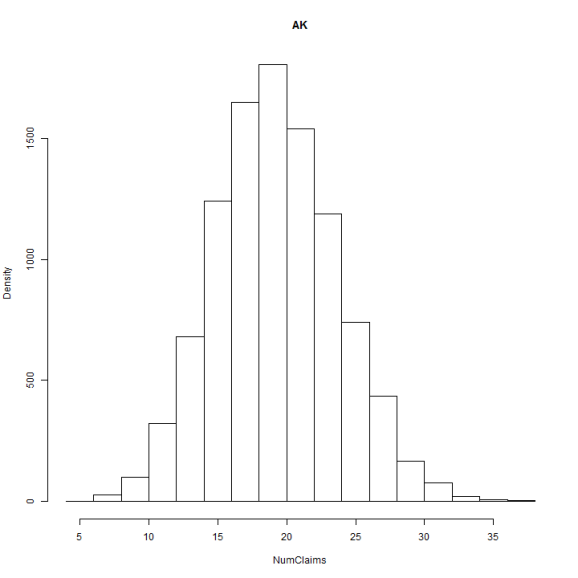
That's enough variation to keep me happy. So, what does the fit look like? I'll first fit a single model and then individual models.

fitPool = glm(NumClaims ~ 1, family = poisson, data = dfPolicies)
summary(fitPool)

## 
## Call:
## glm(formula = NumClaims ~ 1, family = poisson, data = dfPolicies)
## 
## Deviance Residuals: 
##    Min      1Q  Median      3Q     Max  
## -4.239  -2.822  -1.870   0.005  16.185  
## 
## Coefficients:
##             Estimate Std. Error z value Pr(>|z|)    
## (Intercept) 2.195719   0.000472    4654   <2e-16 ***
## ---
## Signif. codes:  0 '***' 0.001 '**' 0.01 '*' 0.05 '.' 0.1 ' ' 1
## 
## (Dispersion parameter for poisson family taken to be 1)
## 
##     Null deviance: 6673372  on 499999  degrees of freedom
## Residual deviance: 6673372  on 499999  degrees of freedom
## AIC: 8248519
## 
## Number of Fisher Scoring iterations: 6

mean(dfPolicies$NumClaims)

## [1] 8.986

exp(coefficients(fitPool))

## (Intercept) 
##       8.986


fitState = glm(NumClaims ~ 0 + Postal, family = poisson, data = dfPolicies)

mean(dfPolicies$NumClaims[dfPolicies$Postal == "AK"])

## [1] 19.75

exp(coefficients(fitState)[1])

## PostalAK 
##    19.75

Note that in this very simple example, the pooled fit gives a lambda parameter equal to the sample mean. By the same token, the model which has a different parameter for every state produces a parameter equal to the sample mean for that state. (Careful with the indexing. Using the postal code as a variable means that it will be re-sorted.)

To fit a model which is a blend between the individual and pooled data, I'll need to the lme4 package.

library(lme4)
fitBlended = glmer(NumClaims ~ 1 + (1 | Postal), family = "poisson", data = dfPolicies)
AK = coefficients(fitBlended)
AK = AK$Postal
AK = AK[[1]][1]
exp(AK)
mean(dfPolicies$NumClaims[dfPolicies$Postal == "AK"])

Note that now the estimated number of claims does NOT equal the sample mean. (It’s barely different and isn’t, when rounded to two decimal places. WordPress and/or knitr truncated the output and I’ve not shown it.) I'll admit that I've lost track of the overall intercept parameter, but I may recall how to fetch that by the morning. I'll also note that the AIC is actually higher using this blended model, so the model is not any better than fitting states individually. (Put differently, each state has 100% credibility.) This is likely because the “between” variance is much, much higher than the “within” variance. I'll try to play with that a bit later.

Tomorrow: It's possible that I've got nothing left to say. Anyone who can provide me with a data set which has film roles and co-stars for Michael Caine and Kevin Bacon will get a free case of beer.

sessionInfo()

## R version 3.0.2 (2013-09-25)
## Platform: x86_64-w64-mingw32/x64 (64-bit)
## 
## locale:
## [1] LC_COLLATE=English_United States.1252 
## [2] LC_CTYPE=English_United States.1252   
## [3] LC_MONETARY=English_United States.1252
## [4] LC_NUMERIC=C                          
## [5] LC_TIME=English_United States.1252    
## 
## attached base packages:
## [1] stats     graphics  grDevices utils     datasets  methods   base     
## 
## other attached packages:
## [1] knitr_1.5        RWordPress_0.2-3 lme4_1.0-5       Matrix_1.1-0    
## [5] lattice_0.20-23 
## 
## loaded via a namespace (and not attached):
##  [1] evaluate_0.5.1 formatR_0.10   grid_3.0.2     MASS_7.3-29   
##  [5] minqa_1.2.1    nlme_3.1-111   RCurl_1.95-4.1 splines_3.0.2 
##  [9] stringr_0.6.2  tools_3.0.2    XML_3.98-1.1   XMLRPC_0.3-0