Introduction

The Ideal Gas Law, , is a very simple yet useful relationship that describes the behaviours of many gases pretty well in many situations.  It is “Ideal” because it makes some assumptions about gas particles that make the math and the physics easy to work with; in fact, the simplicity that arises from these assumptions allows the Ideal Gas Law to be easily derived from the kinetic theory of gases.  However, there are situations in which those assumptions are not valid, and, hence, the Ideal Gas Law fails.

Boyle’s law is inherently a part of the Ideal Gas Law.  It states that, at a given temperature, the pressure of an ideal gas is inversely proportional to its volume.  Equivalently, it states the product of the pressure and the volume of an ideal gas is a constant at a given temperature.

An Example of The Failure of the Ideal Gas Law

This law is valid for many gases in many situations, but consider the following data on the pressure and volume of 1.000 g of oxygen at 0 degrees Celsius.  I found this data set in Chapter 5.2 of ”General Chemistry” by Darrell Ebbing and Steven Gammon.

               Pressure (atm)      Volume (L)              Pressure X Volume (atm*L)
[1,]           0.25                2.8010                  0.700250
[2,]           0.50                1.4000                  0.700000
[3,]           0.75                0.9333                  0.699975
[4,]           1.00                0.6998                  0.699800
[5,]           2.00                0.3495                  0.699000
[6,]           3.00                0.2328                  0.698400
[7,]           4.00                0.1744                  0.697600
[8,]           5.00                0.1394                  0.697000

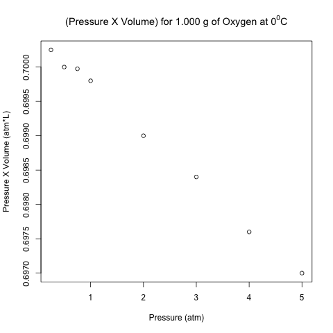
The right-most column is the product of pressure and temperature, and it is not constant.  However, are the differences between these values significant, or could it be due to some random variation (perhaps round-off error)?

Here is the scatter plot of the pressure-volume product with respect to pressure.

These points don’t look like they are on a horizontal line!  Let’s analyze these data using normal linear least-squares regression in R.

> linear.regression.pv.pressure = lm(pressure.times.volume~pressure)
> summary(linear.regression.pv.pressure)

Call:
lm(formula = pressure.times.volume ~ pressure)

Residuals:
       Min         1Q     Median         3Q        Max 
-8.380e-05 -5.054e-05  1.092e-05  4.946e-05  6.411e-05 

Coefficients:
              Estimate Std. Error  t value Pr(>|t|)    
(Intercept)  7.004e-01  3.578e-05 19578.59  < 2e-16 ***
pressure    -6.916e-04  1.354e-05   -51.09 3.77e-09 ***
---
Signif. codes:  0 ‘***’ 0.001 ‘**’ 0.01 ‘*’ 0.05 ‘.’ 0.1 ‘ ’ 1 

Residual standard error: 6.327e-05 on 6 degrees of freedom
Multiple R-squared: 0.9977, Adjusted R-squared: 0.9973 
F-statistic:  2610 on 1 and 6 DF,  p-value: 3.772e-09

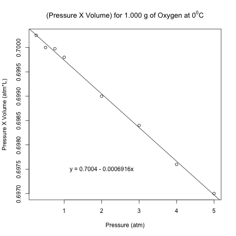
Even though the magnitude of the slope is only 0.0006916, the p-value of the slope shows that there is strong evidence that the product of pressure and volume is not constant with respect to pressure.  Here is the same scatter plot above with the regression line added.  Note how I used the abline() and text() functions to add the line and the equation of the regression line, respectively.  As usual, I used png() and dev.off() to save the image to my folder of choice.

png('INSERT YOUR DIRECTORY PATH HERE/regression pv vs pressure.png')
plot(pressure, pressure.times.volume, main = expression("(Pressure X Volume) for 1.000 g of Oxygen at 0"^0*"C"), ylab = 'Pressure X Volume (atm*L)', xlab = 'Pressure (atm)')
abline(linear.regression.pv.pressure)
text(2, 0.6975, 'y = 0.7004 - 0.0006916x')
dev.off()

This example for oxygen is consistent with experimental results for many other gases, which show that

- the Ideal Gas Law holds well for low pressures and moderate temperatures

- the Ideal Gas Law fails at high pressures and low temperatures

Examining the Postulates of the Kinetic Theory of Gases – Why and When They Fail

Let’s go back to the assumptions of the kinetic theory of gases to see which assumptions may not hold under high pressures or low temperatures.  Here are 2 key ones (numbered as #1 and #3 in Chapter 5 of “General Chemistry” by Darrell Ebbing and Steven Gammon).

Postulate #1: The volume of space occupied by gas particles is negligible compared with the total gas volume.  This allows the theory to model the gas particles as freely moving throughout the entire volume of the gas.  At low pressures, the volume of the individual gas particles is negligible compared to the total volume of the gas, .  However, at high pressures, the particles are closer to and collide with each other more frequently, so their individual volume becomes more important; the space through which the particle moves becomes significantly different from .

Postulate #3: The forces of attraction between the gas particles (i.e. the intermolecular forces) in a gas are weak or negligible.

• At low pressures, the particles are farther apart, so these intermolecular forces are very weak, and this postulate holds well.  At high pressures, the gas particles are closer together, so these intermolecular forces are strong enough to affect the collisions of the molecules and pull them slightly away from the walls of the container.  This reduces the pressure that the gas exerts on the container’s walls.
• At high temperatures, the particles move too fast for the weak intermolecular forces to be attracted by them.  However, at low temperatures, the molecules are moving slower – slow enough that they start to become attracted to nearby molecules.  

In a later post, I will discuss the van der Waals equation, which incorporates these deviations from the ideal assumptions of the kinetic theory of gases to modify the Ideal Gas Law.

Reference:

Chapter 5, Sections 2 and 8.  ”General Chemistry” by Darrell Ebbing and Steven Gammon.  6th Edition, 1999.