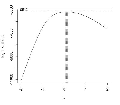
In the previous post, I forgot to show an example of Box-Cox transformation when there’s a lack of normality. The Box-Cox procedure computes values of which best “normalises” the errors.

value	Transformed value of Y
2
1
0.5
0
-0.5
-1
-2

For example:

lm.wpc2 <- lm(wpc ~ vag_disch + milk120 + milk120.sq, data = daisy3)
library(MASS)
boxcox(lm.wpc2, plotit = TRUE)

The plot indicates a log transformation.

Matrix Representation
We can use a matrix representation of the regression equation. The regression equation can be written as where , , and
.

With the following regression:

lm.wpc3 <- lm(wpc ~ milk120 + hs100_ct, data = daisy3)
(lm.wpc3.sum <- summary(lm.wpc3))

Call:
lm(formula = wpc ~ milk120 + hs100_ct, data = daisy3)

Residuals:
Interval from wait period to conception 
   Min     1Q Median     3Q    Max 
-71.83 -36.57 -15.90  23.86 211.18 

Coefficients:
             Estimate Std. Error t value Pr(>|t|)    
(Intercept) 75.884063   6.115894  12.408   <2e-16 ***
milk120     -0.001948   0.001858  -1.049    0.294    
hs100_ct    18.530340   2.106920   8.795   <2e-16 ***
---
Signif. codes:  0 ‘***’ 0.001 ‘**’ 0.01 ‘*’ 0.05 ‘.’ 0.1 ‘ ’ 1 

Residual standard error: 50.53 on 1522 degrees of freedom
Multiple R-squared: 0.0495,	Adjusted R-squared: 0.04825 
F-statistic: 39.63 on 2 and 1522 DF,  p-value: < 2.2e-16 

anova(lm.wpc3)
Analysis of Variance Table

Response: wpc
            Df  Sum Sq Mean Sq F value Pr(>F)    
milk120      1    4865    4865  1.9053 0.1677    
hs100_ct     1  197512  197512 77.3518 <2e-16 ***
Residuals 1522 3886309    2553                   
---
Signif. codes:  0 ‘***’ 0.001 ‘**’ 0.01 ‘*’ 0.05 ‘.’ 0.1 ‘ ’ 1 

We start by making the X matrix and response :

X <- cbind(1 , daisy3[, c(8, 24)])
# or alternatively: model.matrix(lm.wpc3)
y <- daisy3$wpc

Then we get the :

XX <- t(X) %*% X
# or alternatively: crossprod(X, X)
XX
                     1       milk120      hs100_ct
1           1525.00000     4907834.4     -29.87473
milk120  4907834.39954 16535517546.0 -120696.45468
hs100_ct     -29.87473     -120696.5     576.60900

We calculate the inverse of :

XX.inv <- solve(t(X) %*% X)
# or alternatively: qr.solve(XX)
# or also: lm.wpc3.sum$cov.unscaled
XX.inv
                     1       milk120      hs100_ct
1         1.464864e-02 -4.348902e-06 -1.513557e-04
milk120  -4.348902e-06  1.351675e-09  5.761289e-08
hs100_ct -1.513557e-04  5.761289e-08  1.738495e-03

Now to get the coefficients estimates:

XX.inv %*% t(X) %*% y
# or alternatively: solve(t(X) %*% X, t(X) %*% y)
# or also: XX.inv %*% crossprod(X, y)
# or: qr.solve(X, y)
                 [,1]
1        75.884062540
milk120  -0.001948437
hs100_ct 18.530340385

The fitted values:

crossprod(t(X), qr.solve(X, y)

SSE and MSE;

SSE <- crossprod(y, y) - crossprod(y, yhat)
SSE
        [,1]
[1,] 3886309
 
MSE <- SSE / (length(y) - 3)
MSE
         [,1]
[1,] 2553.423

The residual standard error:

sqrt(sum(lm.wpc3$res^2) / (1525 - 3))

The standard errors of the coefficients and the :

sqrt(diag(XX.inv)) * 50.5314
          1     milk120    hs100_ct 
6.115893490 0.001857794 2.106920139

1 - sum(lm.wpc3$res^2) / sum((y - mean(y))^2)
[1] 0.04949679