
Why cost and fuel efficiency are unrelated: Uncorrelated manifest variables can share the same latent causes
[This article was first published on Industrial Code Workshop, and kindly contributed to R-bloggers]. (You can report issue about the content on this page here)
Want to share your content on R-bloggers? click here if you have a blog, or here if you don't.
Want to share your content on R-bloggers? click here if you have a blog, or here if you don't.
In structural equation modelling, we are typically proposing theoretical causes of observed phenomena. These are termed “latent” (the unobserved causes) and manifest (the observed variables we measure, otherwise known as data). Importantly, the theoretical causes of behavior need not have a structure remotely resembling the correlations observed in the data. You might have hundreds of columns of correlated measures, and they might be modelled well by a single latent trait. You might have 30 measured traits, but make the testable prediction that they are best explained by just five uncorrelated latent causes. The case for this posting is a bit unusual: Can two observed variables predicted to share the same latent causes (i.e., that the causes of one observed variable also cause the other) and yet see zero correlation between them at the observed level… This recently came up in a review of some work we’ve been doing, and the answer is “yes: you can”. I thought I’d write down how, using R and some simulations to make this more concrete. In our example, we theorised that religiosity has its roots in two more general, biological systems: subserving community integration, and existential uncertainty. We found support for this model, but it lead to an apparently paradoxical conclusion: the observed manifestation of one of our purported (partial) causes of religiosity, namely existential uncertainty, showed almost no relationship to religiosity. How could these (or any two) measures be completely independent if they share a common cause? The answer lies in countervailing effects: Each of the manifests is the sum of its influences, and, under not-so-uncommon-as-you-might-think instances, these can cancel out. Let’s consider the example of three measures of vehicles (a very R-friendly example, given the ubiquity of mtcars 🙂 Let’s also posit a theoretical model: First that the more cylinders a car has, the more horsepower it can generate, the worse its mpg will be, and the more it will cost to build. Second, that streamlining increases fuel efficiency, but also increases the cost to build, which is reflected in the cost to buy. Assume you’ve gone and collected a large representative set of data, called myCovData. In OpenMx, we can build this model as: library(“OpenMx”) # I use some helper functions: thanks to Hans for the code to readily import them from Github, by writing a source function that handles https… why doesn’t R do this out of the box? url <- https:="" master="" p="" raw.github.com="" tbates="" umx.lib.r="" umx="">source_https <- function="" p="" u="" unlink.tmp.certs="F)"> # read script lines from website using a security certificate require(RCurl) if(!file.exists(“cacert.pem”)){ download.file(url = “http://curl.haxx.se/ca/cacert.pem”, destfile = “cacert.pem”) } script <- cainfo="cacert.pem" followlocation="T," p="" rcurl::geturl="" u=""> if(unlink.tmp.certs) unlink(“cacert.pem”) # parse lines and evaluate in the global environement eval(parse(text = script), envir = .GlobalEnv) } source_https(url) # Using unlink.tmp.certs = T will delete the security certificates text file that source_https downloads |
manifests = c(“HP”, “MPG”, “COST”)
latents = c(“Cylinders”, “Streamlining”)
m1 <- color="#c2c77b" font="" mxmodel="">“m1”, type=“RAM”,
manifestVars = manifests,
latentVars = latents,
# Factor loadings
mxPath(from = “Cylinders” , to = manifests),
mxPath(from = “Streamlining”, to = c(“MPG”,“COST”)),
mxPath(from = manifests, arrows = 2), # manifest residuals
mxPath(from = latents, arrows = 2, free = F, values = 1), #fix latents@1
mxData(myCovData, type = “cov”, numObs = 1000)
)
m1 = mxRun(m1)
summary(m1)
You can visualise this model (here shown with some estimated parameters):
umxGraph_RAM(m1, std=T, precision=2, dotFilename=“name”) # helper function
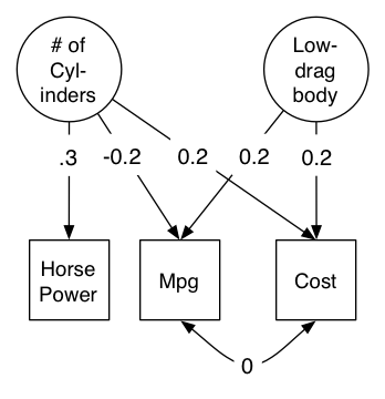
Three manifest (measured) traits of vehicles, modelled as resulting from two (unmeasured) latent traits: The number of cylinders in the engine, and the aerodynamic “slipperiness” of the body. Despite Mpg and Cost sharing the same causes, the manifest correlation between them is zero.
And there’s the conundrum: we can set the correlation between Mpg and Cost to zero without loss of fit. But one can readily see how this emerges in the vehicle example: Big engines are expensive, and lower fuel efficiency (opposite effects on the two variables that we are most interested in) while streamlining induces a positive correlation between our two measures. So, one factor is inducing a positive relationship between Mpg and Cost, and a second is inducing an (equal in this case) negative correlation. The net effects can vary widely, and a zero observed correlation tells us nothing about the presence or absence of shared mechanisms.
We can approach the problem from the other end: To generate the observed data from the theory instead of testing the theory using an SEM.
Here we make 1000 runs of a simulation where we generate the latent causes, then construct a manifest world consisting of 5000 observations of our three manifests from these latent causes, and examine, empirically, the correlation we get on each of those 1000 simulations:
# Uncorrelated manifest variables which share the same latent causes
sim = 100; r = rep(NA,sim)
for (i in 1:sim) {
n = 5000
cyl = rnorm(n = n)
drag = rnorm(n = n)
hp = (.3 * cyl) + .7 * rnorm(n = n)
mpg = (–.2 * cyl) + (.2 * drag) + .6 * rnorm(n = n)
cost = ( .2 * cyl) + (.2 * drag) + .6 * rnorm(n = n)
r[i] = cor(mpg,cost)
}
myCovData = cov(data.frame(HP=hp, MPG= mpg, COST=cost))
hist(r, breaks=40)
text(.02, 50, paste(“mean r =”,prettyNum(mean(r),digits=2)),cex = .8)
Graphically you can see the observed correlations cluster close to zero:
 |
| Correlation (r) of Miles per Gallon (mpg) and Cost of a Car. |
To leave a comment for the author, please follow the link and comment on their blog: Industrial Code Workshop.
R-bloggers.com offers daily e-mail updates about R news and tutorials about learning R and many other topics. Click here if you're looking to post or find an R/data-science job.
Want to share your content on R-bloggers? click here if you have a blog, or here if you don't.