The links to previous parts are listed here. (Part 1, Part 2, Part 3). In this part, I tried to recreate the examples in sections A.3.1 of the computational appendix in the reaction engineering book (by Rawlings and Ekerdt).

Solving a system of ordinary differential equations

This example involves reaction (Benzene pyrolysis) in a plug flow reactor. The actual reactions happening are:

The rate of each reaction is given by:

The feed to the reactor consists of 60kmol/hr of Benzene (B). The temperature of the reactor is and the pressure is .The rate constants and equilibrium constants for this example are:

# Appendix A.3.1: Solution of Differential Equations

# Benzene pyrolysis example

# Parameters
# NBf - feed benzene rate - mol/h
# R - Universal gas constant
# T - Reactor temperature K
# P - Reactor pressure atm
# k1 - rxn1 forward rate constant L/mol.h
# k2 - rxn2 forward rate constant L/mol.h
# Keq1 - rxn1 equilibrium constant
# Keq2 - rxn2 equilibrium constant
pars=c(
NBf=60e3,
R=0.08205,
T=1033,
P=1,
k1=7e5,
k2=4e5,
Keq1=0.31,
Keq2=0.48
)

The governing equations for conversion versus volume in a plug flow reactor is based on extent of each of the reactions:

The initial conditions (corresponding to feed conditions ) are that the extent of reaction is zero.

The flow rates of each component along the reactor volume can be calculated from reaction extent

These are setup in a function that can be passed to an ODE solver. In this case the ODE solver we use is lsode from the R package deSolve. The inputs to the function are:

• Variable over which the integration is done (Volume in this case)
• The state variables of the system (Extent of the two reactions)
• Parameters that are needed for description of the system (Rate constants, Temperature, Pressure, etc.)

The output from this function is the rate of change as described by the equations previously.

# load library deSolve for solving ODEs
library(deSolve)

# function that will be passed to odesolver
# vol is the variable over which the system is integrated (equivalent of time in batch reactions)
# ext is the extent of reactions 1 and 2
# params are the parameters passed to the system
rxnrate=function(vol,ext,params) {
    with(as.list(c(ext,params)),{
      NB=NBf-2*ext1-ext2
      ND=ext1-ext2
      NH=ext1+ext2
      NT=ext2
      Q=NBf*R*T/P
      cB=NB/Q
      cD=ND/Q
      cT=NT/Q
      cH=NH/Q
      dext1=k1*(cB*cB-cD*cH/Keq1)
      dext2=k2*(cB*cD-cT*cH/Keq2)
      return(list(c(dext1=dext1,dext2=dext2)))
    })
}

Since the reaction start only after the feed enters the reactor, the extent of reaction is zero for both reactions at the beginning of the reactor (V=0L). The set of volumes where the concentration and reaction extent is computed is chosen in this case to be from 0L to 1600L at every 50L. The ODE solver lsode from deSolve package is used to solve the system of equations.

# initial extent of reaction (zero in this case for both reactions)
extinit=c(ext1=0,ext2=0)
# Volumes where the concentration is reported (in this case 0 to 1600L at every 50L)
vols=seq(0,1600,length=50)
# Solution of the set of differential equations using lsode solver in deSolve package
extout=lsode(times=vols,y=extinit,func=rxnrate,parms=pars)

extout contains the extent of reaction vs volume data. That is used to compute mole fraction and conversion at different volumes along the reactor.

# Calculation of mole fraction and conversion from extent of reaction at different volumes
extoutdf=data.frame(extout)
NBf=pars["NBf"]
extoutdf$conv=(extoutdf$ext1*2+extoutdf$ext2)/NBf
extoutdf$yB=(NBf-2*extoutdf$ext1-extoutdf$ext2)/NBf
extoutdf$yD=(extoutdf$ext1-extoutdf$ext2)/NBf
extoutdf$yT=(extoutdf$ext2)/NBf
extoutdf$yH=(extoutdf$ext1+extoutdf$ext2)/NBf

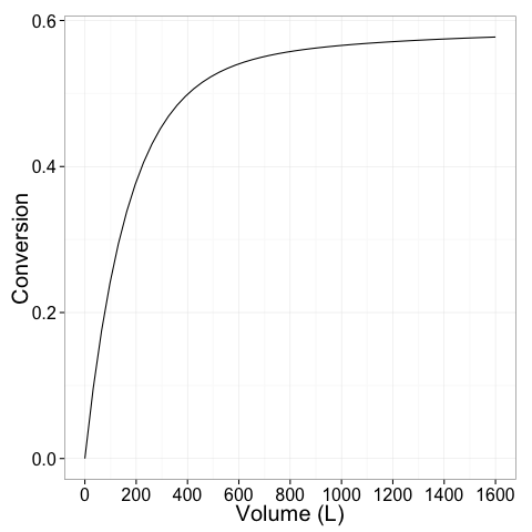
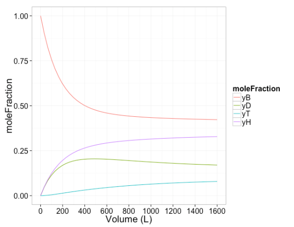
Next conversion and mole fraction is plotted as a function of reaction volume

# load library ggplot2 for plotting
library(ggplot2)
# load library reshape2 for data reshaping
library(reshape2)
# plot of conversion vs volume
ggplot(extoutdf,aes(x=time,y=conv))+geom_line()+
scale_x_continuous(breaks=seq(0,1600,by=200))+xlab('Volume (L)')+ylab('Conversion')+theme_bw(20)

# plot of mole fraction vs volume
tmp=melt(extoutdf[,c("time","yB","yD","yT","yH")],id.vars=c("time"),variable.name="moleFraction")
ggplot(tmp,aes(x=time,y=value,color=moleFraction))+geom_line()+
scale_x_continuous(breaks=seq(0,1600,by=200))+xlab('Volume (L)')+ylab('moleFraction')+theme_bw(20)

sessionInfo()
R version 2.15.1 (2012-06-22)
Platform: i386-apple-darwin9.8.0/i386 (32-bit)

locale:
[1] en_US.UTF-8/en_US.UTF-8/en_US.UTF-8/C/en_US.UTF-8/en_US.UTF-8

attached base packages:
[1] stats     graphics  grDevices utils     datasets  methods   base

other attached packages:
[1] reshape2_1.2.1  ggplot2_0.9.2.1 deSolve_1.10-4

loaded via a namespace (and not attached):
[1] colorspace_1.1-1   dichromat_1.2-4    digest_0.5.2       grid_2.15.1
[5] gtable_0.1.1       labeling_0.1       MASS_7.3-18        memoise_0.1
[9] munsell_0.3        plyr_1.7.1         proto_0.3-9.2      RColorBrewer_1.0-5
[13] scales_0.2.2       stringr_0.6.1