Students in any basic statistics class are taught linear regression, which is one of the simplest forms of a statistical model. The basic idea is that a ‘response’ variable can be mathematically related to one or any number of ‘explanatory’ variables through a linear equation and a normally distributed error term. With any statistical tool, linear regression comes with a set of assumptions that have to be met in order for the model to be valid. These assumptions include¹:

• model residuals are individually normally distributed
• constant variance or homogeneity (i.e., even spread of residuals)
• explanatory variables are deterministic
• independence of observations or no pattern in residuals

When I first learned about linear regression I was overly optimistic about how easy it was to satisfy each of these assumptions. Once I learned to be more careful I started using techniques to verify if each of these assumptions were met. However, no one bothered to tell me what actually happens when these assumptions are violated, at least not in a quantitative sense. Most textbooks will tell you that if your model violates these assumptions the statistics or coefficients describing relationships among variables will be biased. In other words, your model will tell you information that is systematically different from relationships describing the true population.

Of course the bias in your model depends on what rule you’ve violated and it would be impractical (for the purpose of this blog) to conduct a thorough analysis of each assumption. However, I’ve always wondered what would happen if I ignored the fourth point above regarding independence. I’ve had the most difficulty dealing with auto-correlation among observations and I’d like to get a better idea of how a model might be affected if this assumption is ignored. For example, how different would the model coefficients be if we created a regression model without accounting for a correlation structure in the data? In this blog I provide a trivial but potentially useful example to address this question. I start by simulating a dataset and show how the model estimates are affected by ignoring spatial dependency among observations. I also show how these dependencies can be addressed using an appropriate model. Before I continue, I have to give credit to the book ‘Mixed Effects Models and Extensions in Ecology with R’¹, specifically chapters 2 and 7. The motivation for this blog comes primarily from these chapters and interested readers should consult them for more detail.

Let’s start by importing the packages gstat, sp, and nlme. The first two packages have some nifty functions to check model assumptions and the nlme package provides models that can be used to account for various correlation structures.

#import relevant packages library(gstat) library(sp) library(nlme)

Next we create a simulated dataset, which allows us to verify the accuracy of our model if we know the ‘true’ parameter values. The dataset contains 400 observations that are each spatially referenced by the ‘lat’ and ‘lon’ objects. The coordinates were taken from a uniform distribution (from -4 to 4) using the runif function. There are two explanatory variables that are both taken from the standard normal distribution using the rnorm function. I’ve used the set.seed function so the results can be reproduced. R uses pseudo-random number generation, which can be handy for sharing examples.

#create simulated data, lat and lon from uniformly distributed variable #exp1 and exp2 from random normal set.seed(2) samp.sz<-400 lat<-runif(samp.sz,-4,4) lon<-runif(samp.sz,-4,4) exp1<-rnorm(samp.sz) exp2<-rnorm(samp.sz)

The response variable is a linear combination of the explanatory variables and follows the form of a standard linear model. I’ve set the parameters for the linear model as 1, 4, -3, and -2 for the intercept and slope values. The error term is also normally distributed. Note that I’ve included latitude in the model to induce a spatial correlation structure.

#resp is linear combination of explanatory variables #plus an error term that is normally distributed resp<-1+4*exp1-3*exp2-2*lat+rnorm(samp.sz)

Setting the parameter values is key because we hope that any model we use to relate the different variables will return values that are very close to the actual and show minimal variation. In the real world, we do not know the actual parameter values so we have to be really careful that we are using the models correctly.

Next, we can plot the variables and run some diagnostics to verify we’ve created appropriate data. Plotting the data frame produces scatterplots that indicate correlation among the simulated variables.

#pair plots of variables plot(data.frame(resp,exp1,exp2,lat))

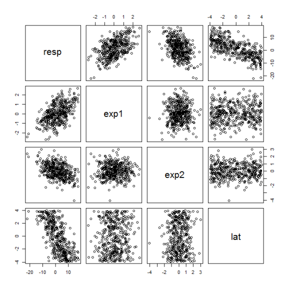
The cor function verifies the info in the figure by returning Pearson correlation coefficients. Note the sign and magnitude of the correlations of the response variable with all other variables. The explanatory variables and latitude are not correlated with each other.

#correlation between variables cor(data.frame(resp,exp1,exp2,lat)) resp exp1 exp2 lat resp 1.0000000 0.53416042 -0.44363892 -0.70131965 exp1 0.5341604 1.00000000 0.01703620 0.03419987 exp2 -0.4436389 0.01703620 1.00000000 0.04475536 lat -0.7013196 0.03419987 0.04475536 1.00000000

Now that we’ve simulated our data, we can create a linear model to see if the parameter coefficients are similar to the actual. In this example, we’re ignoring the spatial correlation structure. If we were savvy modelers, we would check for spatial correlation prior to building our model. Spatial correlation structures in actual data may also be more complex than a simple latitudinal gradient, so we need to be extra careful when evaluating the independence assumption. We create the model using the basic lm function.

mod<-lm(resp~exp1+exp2) coefficients(summary(mod)) Estimate Std. Error t value Pr(>|t|) (Intercept) 1.298600 0.2523227 5.146587 4.180657e-07 exp1 3.831385 0.2533704 15.121673 4.027448e-41 exp2 -3.237224 0.2561525 -12.637879 5.276878e-31

The parameter estimates are not incredibly different form the actual values. Additionally, the standard errors of the estimates are not large enough to exclude the true parameter values. We can verify this using a t-test with the null hypothesis for each parameter set at the actual (the default null in lm is zero). I’ve created a function for doing this that takes the observed mean value as input rather than the normal t.test function that uses a numeric vector of values as input. The arguments for the custom function are the observed mean (x.bar), null mean (mu), standard error (se), degrees of freedom (deg.f), and return.t which returns the t-statistic if set as true.

#function for testing parameter values against actual t_test<-function(x.bar,mu,se,deg.f,return.t=F){ if(return.t) return(round((x.bar-mu)/se,3)) pt(abs((x.bar-mu)/se),deg.f,lower.tail=F)*2 } #for first explanatory variable t_test(3.8314, 4, 0.2534, 397) [1] 0.5062122

The p-value indicates that the estimated parameter value for the first explanatory variable is not different from the actual. We get similar results if we test the other parameters. So far we’ve shown that if we ignore the spatial correlation structure we get fairly reasonable parameter estimates. Can we improve our model if we account for the spatial correlation structure?

Before we model spatial correlation we first have to identify its existence (remember, we’re assuming we don’t know the response is correlated with latitude). Let’s dig a little deeper by first describing some tools to evaluate the assumption of independence. The easiest way to evaluate this assumption in a linear model is to plot the model residuals by their spatial coordinates. We would expect to see some spatial pattern in the residuals if we have not accounted for spatial correlation. The bubble plot function in the sp package can be used to plot residuals.

dat<-data.frame(lon,lat,resids=resid(mod)) coordinates(dat)<-c('lon','lat') bubble(dat,zcol='resids')

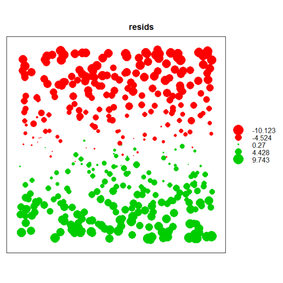
A nice feature of the bubble function is that it color codes the residuals based on positive and negative values and sets the size of the points in proportion to the magnitude. An examination of the plot shows a clear residual pattern with latitude such that smaller values are seen towards the north.

The bubble plot provides a qualitative means of evaluating spatial correlation. A more quantitative approach is to evaluate semivariance, which provides a measure of spatial correlation between points at different distances. Points closer to one another are more likely to be similar if observations in our dataset are spatially correlated. The variety of statistics that can be applied to spatial data is staggering and evaluations of semivariance are no exception. For this example, it is sufficient to know that points closer to one another will have smaller values of semivariance (more similar) and those farther apart will have larger values (less similar) if points are spatially correlated. We would also expect calculated values of semivariance to vary depending on what direction we are measuring (i.e., anisotropy). For example, we might not detect spatial correlation if we estimate semivariance strictly in an east to west direction, whereas semivariance would vary quite dramatically along a north to south direction. We can apply the variogram function (gstat package) to estimate semivariance and also account for potential differences depending on direction.

var.mod<-variogram(resids~1,data=dat,alpha=c(0,45,90,135)) plot(var.mod)

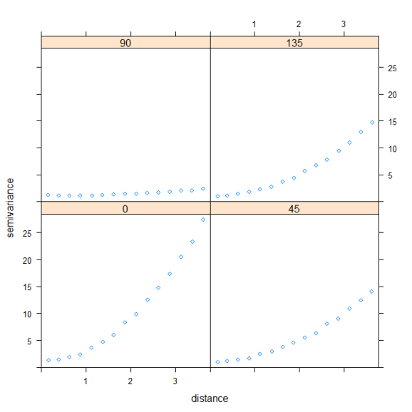
When we use the variogram function we can specify directions in which semivariance is measured using the alpha argument. Here we’ve specified that we’d like to measure semivariance in the residuals in a northern, north-eastern, eastern, and south-eastern direction. This is the same as estimating semivariance in directions 180 degrees from what we’ve specified, so it would be redundant if we looked at semivariance in a southern, south-western, western, and north-western direction. The plot shows that spatial correlation is strongest in a north-south direction and weakest along an east-west direction, which confirms the latitudinal change in our response variable.

Our analyses have made it clear that the model does not account for spatial correlation, even though our parameter estimates are not significantly different from the actual values. If we account for this spatial correlation can we improve our model? An obvious solution would be to include latitude as an explanatory variable and obtain a parameter estimate that describes the relationship. Although this would account for spatial correlation, it would not provide any explanation for why our response variable changes across a latitudinal gradient. That is, we would not gain new insight into causation, rather we would only create a model with more precise parameters. If we wanted to account for spatial correlation by including an additional explanatory variable we would have to gather additional data based on whatever we hypothesized to influence our response variable. Temperature, for example, may be a useful variable because it would likely be correlated with latitude and its relationship with the response variable could be biologically justified.

In the absence of additional data we can use alternative models to account for spatial correlation. The gls function (nlme package) is similar to the lm function because it fits linear models, but it can also be used to accommodate errors that are correlated. The implementation is straightforward with the exception that you have specify a form of the spatial correlation structure. Identifying this structure is non-trivial and the form you pick will affect how well your model accounts for spatial correlation. There are six options for the spatial correlation structure. Picking the optimal correlation structure requires model comparison using AIC or similar tools.

For our example, I’ve shown how we can create a model using only the Gaussian correlation structure. Also note the form argument, which can be used to specify a covariate that captures the spatial correlation.

#refit model with correlation structure mod.cor<-gls(resp~exp1+exp2,correlation=corGaus(form=~lat,nugget=TRUE)) summary(mod.cor) Coefficients: Value Std.Error t-value p-value (Intercept) 154.49320 393.3524 0.39276 0.6947 exp1 3.99840 0.0486 82.29242 0.0000 exp2 -3.01688 0.0491 -61.38167 0.0000

The gls function seems to have trouble estimating the intercept. If we ignore this detail, the obvious advantage of accounting for spatial correlation is a reduction in the standard error for the slope estimates. More precisely, we’ve reduced the uncertainty of our estimates by over 500% from those obtained using lm, even though our initial estimates were not significantly different from the actual.

The advantage of accounting for spatial correlation is a huge improvement in the precision of the parameter estimates. Additionally, we do not sacrifice degrees of freedom if we use the gls function to model spatial correlation. Hopefully this example has been useful for emphasizing the need to account for model assumptions. I invite further discussion on methods for modeling spatial correlation.

Get the code here:

¹Zuur, A.F., Ieno, E.N., Walker, N.J., Saveliev, A.A., Smith, G.M., 2009. Mixed Effects Models and Extensions in Ecology with R. Springer, New York.