
Great Circles, Black Holes, and Community Events Part 2 of 3
[This article was first published on OutLie..R, and kindly contributed to R-bloggers]. (You can report issue about the content on this page here)
Want to share your content on R-bloggers? click here if you have a blog, or here if you don't.
Want to share your content on R-bloggers? click here if you have a blog, or here if you don't.
This post will examine the Heber Valley Railroad, a small town tourist attraction using event gravitational pull. Using the information from part 1 the two factors associated with the events gravity, the number of participants, and the distance they traveled. The number of participants can be shown using bar charts, histograms, and summary tables. The distance traveled can be displayed using bar charts, histograms, summary charts, and most important great circle maps. Below are some of the charts I created when doing the analysis.
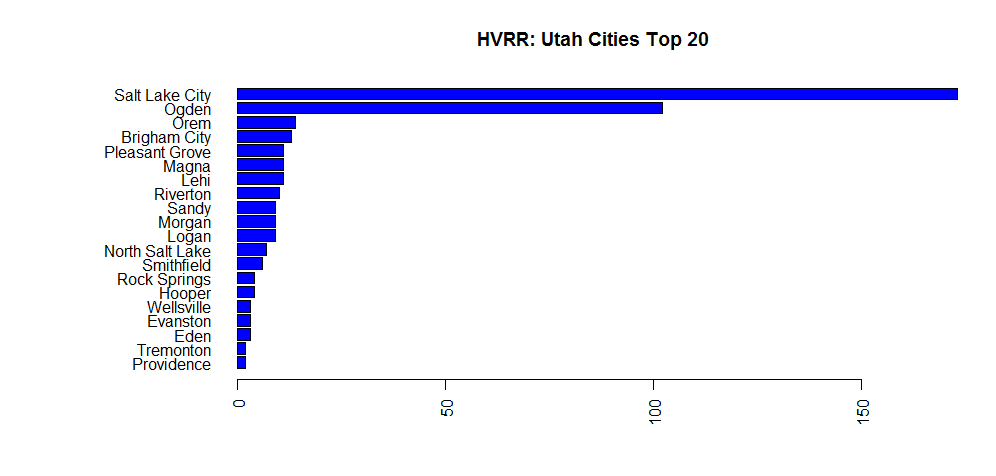
The first two are bar charts show where the majority of train riders are coming from. From the graphs Salt Lake City Utah is number one, followed by Ogden, then it goes down hill from there very quickly. The purpose of these first graphs is to show how many people are coming to the event and where.
The first two are bar charts show where the majority of train riders are coming from. From the graphs Salt Lake City Utah is number one, followed by Ogden, then it goes down hill from there very quickly. The purpose of these first graphs is to show how many people are coming to the event and where.

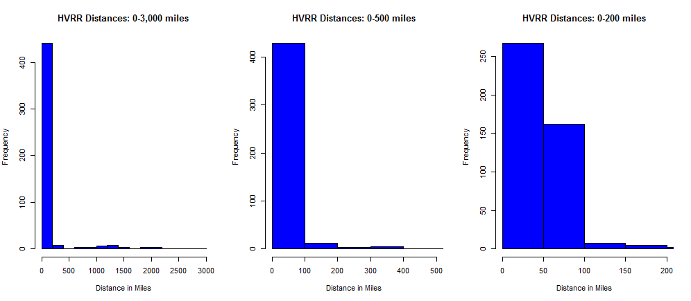
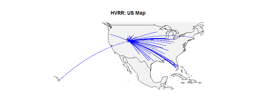
Where the first set of graphs show the cities, the histograms show where people are coming from in terms of distance. The first histogram shows all the data, the next two are zoomed in to show the majority of people travel less than 100 miles (as the crow flies) to get to the train. While the majority of people who ride the train do so within 100 miles, there are many who travel many miles. But it should be noted, there are only 1-3 customers per line. The map looks really good, but the majority of those traveling long distances, are much fewer.
While the map shows a number of people coming from various locations, there are only 1-3 people per line, nothing to really spend any marketing funds to. The map does show how far people do come.
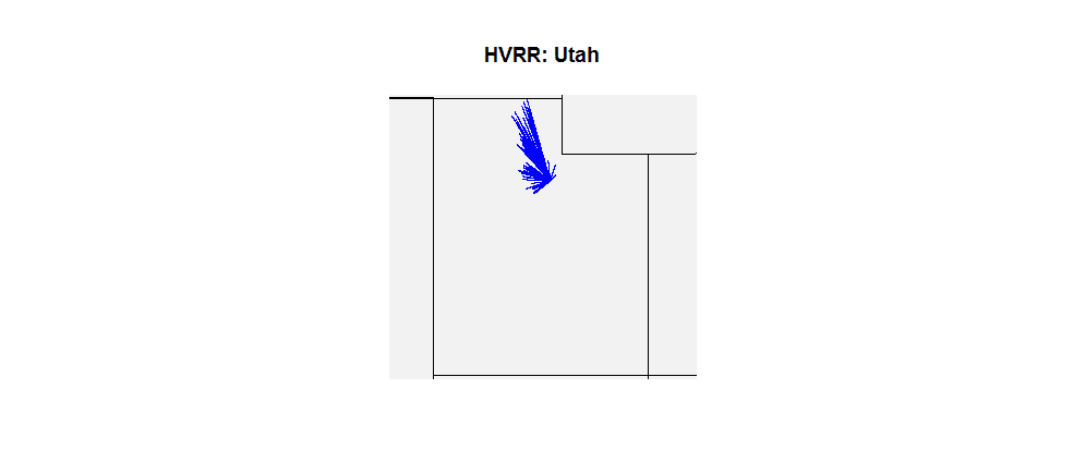
The next two maps show that within Utah the majority of people riding the train come from Salt Lake, Ogden, and the Wasatch Front area.
require(geosphere)
require(maps)

#HVRR Analysis
#Step 1: basic Stats. Summaries, Histograms, bar charts
#reading the file in

hvrr<-read.table(file.choose(), header=TRUE)

#summary stats
summary(hvrr)

#histograms
par(mfrow=c(1,2))
label.1<-c(‘Utah (424 88%)’, ‘Other(58 12%)’)
state<-c(424, 58)
barplot(state, names.arg=label.1, main=‘HVRR: States’, col=‘blue’)
label.2<-c(‘Salt Lake’, ‘Ogden’, ‘Other’)
cities<-c(173, 102, 149)
barplot(cities, names.arg=label.2, main=‘HVRR: Cities Within Utah’, col=‘blue’)
par(las=2, mar=c(5,12,4,2), mfrow=c(1,1))
city.1<-sort(table(hvrr$city))
city.1<-tail(city.1, n=20)
barplot(city.1, col=‘blue’, hor=TRUE, main=‘HVRR: Utah Cities Top 20’)
par(las=0, mar=c(5,4,4,2))

#distance analysis
heber<-c(-111.33259, 40.511413)
data<-matrix(data=c(hvrr$long, hvrr$lat), nrow=482, ncol=2)
ut<-subset(hvrr, subset=(st==‘UT’))
data.ut<-matrix(data=c(ut$long, ut$lat), nrow=424, ncol=2)
dist<-(distm(heber, data, fun=distVincentyEllipsoid)*0.000621371192)
dist.rr<-matrix(dist, nrow=482, ncol=1)
hvrr<-cbind(hvrr, dist.rr)

#histograms of various shapes and zooms
summary(dist.rr)
par(mfrow=c(1, 3))
hist(dist.rr, breaks=12, main=‘HVRR Distances: 0-3,000 miles’, xlab=‘Distance in Miles’, col=‘blue’)
hist(dist.rr, breaks=24, main=‘HVRR Distances: 0-500 miles’, xlab=‘Distance in Miles’, xlim=c(0, 500), col=‘blue’)
hist(dist.rr, breaks=50, main=‘HVRR Distances: 0-200 miles’, xlab=‘Distance in Miles’, xlim=c(0, 200), col=‘blue’)
par(mfrow=c(1,1))

#mapping it out

#US
map("world", col="#f2f2f2", fill=TRUE, bg="white", lwd=0.25, xlim=c(-158, -65), ylim=c(15, 50))
title(main=‘HVRR: US Map’)
for(i in 1:dim(data)[1]){
 inter <- gcIntermediate(heber, data[i, 1:2], n=482, addStartEnd=TRUE)
 lines(inter, col="blue")
}

#Zoomed into Utah
par(mfrow=c(1,1), mar=c(5,4,4,2))
map("state", col="#f2f2f2", fill=TRUE, bg="white", lwd=0.25, xlim=c(-115, -108), ylim=c(37, 42))
title(main=‘HVRR: Utah’)
for(i in 1:dim(data.ut)[1]){
 inter <- gcIntermediate(heber, data.ut[i, 1:2], n=424, addStartEnd=TRUE)
 lines(inter, col="blue")
}

#Wasatch Front
map("state", col="#f2f2f2", fill=TRUE, bg="white", lwd=0.25, xlim=c(-112.5, -111), ylim=c(40, 42))
title(main=‘HVRR: Utah- Wasatch Front’)
for(i in 1:dim(data.ut)[1]){
 inter <- gcIntermediate(heber, data.ut[i, 1:2], n=424, addStartEnd=TRUE)
 lines(inter, col="blue")
}
par(mfrow=c(1,1))
To leave a comment for the author, please follow the link and comment on their blog: OutLie..R.
R-bloggers.com offers daily e-mail updates about R news and tutorials about learning R and many other topics. Click here if you're looking to post or find an R/data-science job.
Want to share your content on R-bloggers? click here if you have a blog, or here if you don't.