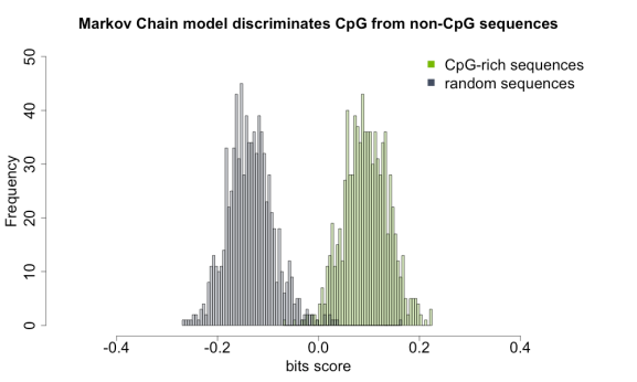
discrimination between CpG islands and random sequences using Markov chains
Want to share your content on R-bloggers? click here if you have a blog, or here if you don't.
Major part of modern research is trying to find patterns in the given dataset using learning methods. One of the methods that can use a priori information for such purpose is Markov chains, in which the probability of symbol occurrence depends only on previous symbol (appropriate for the dinucleotide modeling).
The question I am addressing here is – given the random sequence from mouse genome, can you predict that this is a CpG island? In the next few lines of code you will find many useful approaches to MC modeling, splitting of odd and even elements of R vector using “substring” function, querying the UCSC database solely via R, and informative visualization with transparent histograms.
Note that I got sequences from BSgenome.Mmusculus.UCSC.mm9 library, which contains complete mouse genome. Since the download of the same might be tedious for some (~750mb), I uploaded the cpg and random regions to pastebin.
CpG Islands – http://pastebin.com/372cfs6U
Random – http://pastebin.com/wZyKFFkx
# load libraries
library(compiler)
library(rtracklayer)
library(GenomicFeatures)

# ignore following if you're taking sequences from pastebin
library(BSgenome.Mmusculus.UCSC.mm9)

# models derived by ML estimator (a_st = c_st / sum(c_st')) from CpG and non-CpG islands
# in each row, nucleotide has a probability of being followed by respective base in the column,
# thus rows should sum up to 1

# notice the drop of G being followed by C in negative model (due to C being target of spontaneous deamination upon methylation),
# same is preserved in CpG-islands rich regions due to the lack of methylation supression on promoter regions

positive.model <- t(matrix(
    data  = c(0.180, 0.274, 0.426, 0.120, 0.171, 0.368, 0.274, 0.188, 0.161, 0.339, 0.375, 0.125, 0.079, 0.355, 0.384, 0.182),
    nrow  = 4,
    ncol  = 4,
    dimnames = list(c("A", "C", "G", "T"), c("A", "C", "G", "T"))
))

negative.model <- t(matrix(
    data  = c(0.300, 0.205, 0.285, 0.210, 0.322, 0.298, 0.078, 0.302, 0.248, 0.246, 0.298, 0.208, 0.177, 0.239, 0.292, 0.292),
    nrow  = 4,
    ncol  = 4,
    dimnames = list(c("A", "C", "G", "T"), c("A", "C", "G", "T"))
))

# log-likelihood table derived from log-odds ratio of two models
# used for discrimination of sequences as CpG or non-CpG islands

likelihood.values <- round(log2(positive.model/negative.model), 3)

# score (in bits) of the sequence normalized by its length
bits.score <- function(sequence = DNA_region, model = likelihood.values) {

    # sequence length
    seq.length <- nchar(sequence)

    # if sequence is odd, trim the last element
    if (seq.length %% 2 != 0) {
        sequence   <- paste(strsplit(sequence, split = "")[[1]][-seq.length], collapse = "")
        seq.length <- seq.length - 1
    }

    # extract dinucleotides
    idx   <- seq(1, seq.length)
    odds  <- idx[(idx %% 2) == 1]
    evens <- idx[(idx %% 2) == 0]

    tmp.split <- substring(sequence, odds, evens)

    # return normalized sum of the log-likelihood scores
    return(sum(unlist(lapply(tmp.split, function(tmp.dinucleotide) {
        lookup <- strsplit(tmp.dinucleotide, split = "")[[1]]
        return(model[lookup[1], lookup[2]])
    }))) / seq.length)
}

bits.score <- cmpfun(bits.score)

# setting up the discrimination model
model.score <- function(sequences = DNA_region) {
    all.dinucleotides <- do.call("c", lapply(sequences, function(sequence) {

        # sequence length
        seq.length <- nchar(sequence)

        # if sequence is odd, trim the last element
        if (seq.length %% 2 != 0) {
            sequence   <- paste(strsplit(sequence, split = "")[[1]][-seq.length], collapse = "")
            seq.length <- seq.length - 1
        }

        # extract dinucleotides
        idx   <- seq(1, seq.length)
        odds  <- idx[(idx %% 2) == 1]
        evens <- idx[(idx %% 2) == 0]

        tmp.split <- substring(sequence, odds, evens)
    }))

    all.counts <- t(matrix(table(all.dinucleotides), ncol = 4, nrow = 4, dimnames = list(c("A", "C", "G", "T"), c("A", "C", "G", "T"))))
    all.counts <- t(apply(all.counts, 1, function(tmp.row) { tmp.row / sum(tmp.row) } ))

return(all.counts)
}

model.score <- cmpfun(model.score)

# following code extracts sequences from annotated and random parts of the mm9 genome
# ignore it if you're using pastebin text
# querying the UCSC database for CpG islands track
session               <- browserSession()
genome(session)       <- "mm9"
query                 <- ucscTableQuery(session, "CpG Islands")
cpg.islands           <- getTable(query)
cpg.islands           <- subset(cpg.islands, cpg.islands$chrom == "chr1", select = c("chrom", "chromStart", "chromEnd", "length"))
colnames(cpg.islands) <- c("chr", "region.start", "region.end", "region.width")

# generate random positions via "sample" function, but not exceeding largest width of CpG island
random.regions            <- data.frame(chr = "chr1", region.start = sample(seq(0, seqlengths(Mmusculus)[["chr1"]] - max(cpg.islands$region.width)), nrow(cpg.islands)))
random.regions$region.end <- random.regions$region.start + cpg.islands$region.width

markov.chain.seq <- lapply(c("cpg.islands", "random.regions"),  FUN = function(tmp.sample) {
    tmp.dataset <- get(tmp.sample)

    if (nrow(tmp.dataset) > 0) {
        tmp.sview        <- as.character(DNAStringSet(Views(unmasked(Mmusculus[["chr1"]]), start = tmp.dataset$region.start, end = tmp.dataset$region.end)))
    }

    return(tmp.sview)
})

# only keep sequences from non-repetitive parts of genome
markov.chain.seq        <- lapply(markov.chain.seq, function(tmp.sample) { do.call("c", lapply(tmp.sample, function(tmp.seq) { tmp.seq[!grepl("N", tmp.seq)] })) })
names(markov.chain.seq) <- c("cpg.islands", "random.regions")

# you can substitute "lapply" with "mclapply" for parallel processing with multicore package at this point
# output of the discrimination plot
png("~/MarkovChain.png", 1000, 600)
    hist(unlist(lapply(markov.chain.seq[[1]], bits.score)), breaks = 100, xlim = c(-0.5, 0.5), ylim = c(0, 50), col = "#78B90050", main = "Markov Chain model discriminates CpG from non-CpG sequences", xlab = "bits score")
    hist(unlist(lapply(markov.chain.seq[[2]], bits.score)), breaks = 100, col = "#444D6150", add = TRUE)
legend("topright", c("CpG-rich sequences", "random sequences"), col = c("#78B900", "#444D61"), pch = 15, cex = 2, bty = "n")
dev.off()
Similar to the HMM example from previous post, the Markov chain is also based on Durbin (1998.) book.
Cheers, mintgene.
R-bloggers.com offers daily e-mail updates about R news and tutorials about learning R and many other topics. Click here if you're looking to post or find an R/data-science job.
Want to share your content on R-bloggers? click here if you have a blog, or here if you don't.

