In a previous post I discussed the concept of gradient descent.  Given some recent work in the online machine learning course offered at Stanford,  I’m going to extend that discussion with an actual example using R-code  (the actual code is adapted from a computer science course at Colorado State, and the example is verbatim from the notes here: http://www.cs.colostate.edu/~anderson/cs545/Lectures/week6day2/week6day2.pdf )

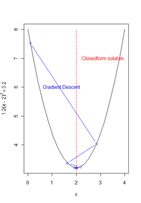
Suppose you want to minimize the function 1.2 * (x-2)^2 + 3.2. Basic calculus requires that we find the 1st derivative and solve for the value of x such that f'(x) = 0. This is easy enough to do, f'(x) = 2*1.2*(x-2). Its easy to see that a value of 2 satisfies f'(x) =  0. Given that the second order conditions hold, this is a minimum.

Its not alwasys the case that we would get a function so easy to work with, and in many cases we may need to numerically estimate the value that minimizes the function. Gradient descent offers a way to do this. Recall from my previous post the gradient descent algorithm can be summarized as follows:

repeat until convergence {
Xn+1 = Xn – α∇F(Xn)  or  x := x – α∇F(x)  (depending on your notational preferences)
}

Where ∇F(x)  would be the derivative we calculated above for the function at hand and α is the learning rate. This can easily be implemented R. The following code finds the values of x that minimize the function above and plots the progress of the algorithm with each iteration. (as depicted in the image below)


R-code:

#  ----------------------------------------------------------------------------------
# |PROGRAM NAME: gradient_descent_R
# |DATE: 11/27/11
# |CREATED BY: MATT BOGARD 
# |PROJECT FILE:              
# |----------------------------------------------------------------------------------
# | PURPOSE: illustration of gradient descent algorithm
# | REFERENCE: adapted from : http://www.cs.colostate.edu/~anderson/cs545/Lectures/week6day2/week6day2.pdf                
# | 
#  ---------------------------------------------------------------------------------
 
xs <- seq(0,4,len=20) # create some values
 
# define the function we want to optimize
 
f <-  function(x) {
1.2 * (x-2)^2 + 3.2
}
 
# plot the function 
plot(xs , f (xs), type="l",xlab="x",ylab=expression(1.2(x-2)^2 +3.2))
 
# calculate the gradeint df/dx
 
grad <- function(x){
  1.2*2*(x-2)
}
 
 
# df/dx = 2.4(x-2), if x = 2 then 2.4(2-2) = 0
# The actual solution we will approximate with gradeint descent
# is  x = 2 as depicted in the plot below
 
lines (c (2,2), c (3,8), col="red",lty=2)
text (2.1,7, "Closedform solution",col="red",pos=4)
 
 
# gradient descent implementation
x <- 0.1 # initialize the first guess for x-value
xtrace <- x # store x -values for graphing purposes (initial)
ftrace <- f(x) # store y-values (function evaluated at x) for graphing purposes (initial)
stepFactor <- 0.6 # learning rate 'alpha'
for (step in 1:100) {
x <- x - stepFactor*grad(x) # gradient descent update
xtrace <- c(xtrace,x) # update for graph
ftrace <- c(ftrace,f(x)) # update for graph
}
 
lines ( xtrace , ftrace , type="b",col="blue")
text (0.5,6, "Gradient Descent",col="blue",pos= 4)
 
# print final value of x
print(x) # x converges to 2.0