
Basic Econometrics in R and SAS
[This article was first published on Econometric Sense, and kindly contributed to R-bloggers]. (You can report issue about the content on this page here)
Want to share your content on R-bloggers? click here if you have a blog, or here if you don't.
Want to share your content on R-bloggers? click here if you have a blog, or here if you don't.
Regression Basics
y= b0 + b1 *X ‘regression line we want to fit’
The method of least squares minimizes the squared distance between the line ‘y’ and
individual data observations yi. 
That is minimize: ∑ ei2 = ∑ (yi – b0 – b1 Xi )2 with respect to b0 and b1 .
This can be accomplished by taking the partial derivatives of ∑ ei2 with respect to each coefficient and setting it equal to zero.
∂ ∑ ei2 / ∂ b0 = 2 ∑ (yi – b0 – b1 Xi ) (-1) = 0
∂ ∑ ei2 / ∂ b1 = 2 ∑(yi – b0 – b1 Xi ) (-Xi) = 0
Solving for b0 and b1 yields the ‘formulas’ for hand calculating the estimates:
b0 = ybar – b1 Xbar
b1 = ∑ (( Xi – Xbar) (yi – ybar)) / ∑ ( Xi – Xbar) = [ ∑Xi Yi – n xbar*ybar] / [∑X2 – n Xbar2]
= S( X,y) / SS(X)
Example with Real Data:
Given real data, we can use the formulas above to derive (by hand /caclulator/excel) the estimated values for b0 and b1, which give us the line of best fit, minimizing ∑ ei2 = ∑ (yi – b0 – b1 Xi )2 .
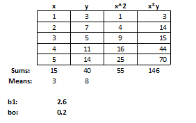
n= 5
∑Xi Yi = 146
∑X2 = 55
Xbar = 3
Ybar =8
b1 = [ ∑Xi Yi – n xbar*ybar] / [∑X2 – n Xbar2] (146-5*3*8)/(55-5*32) = 26/10 = 2.6
b0= ybar – b1 Xbar = 8-2.6*3 = .20
You can verify these results in PROC REG in SAS.
/* GENEARATE DATA */
DATA REGDAT;
INPUT X Y;
CARDS;
1 3
2 7
3 5
4 11
5 14
;
RUN;
/* BASIC REGRESSION WITH PROC REG */
PROC REG DATA = REGDAT;
MODEL Y = X;
RUN;
QUIT;
OUTPUT:

OUTPUT:
Similarly this can be done in R using the ‘lm’ function:
#------------------------------------------------------------
#  regression with canned lm routine
#------------------------------------------------------------

# read in data manually

x <- c(1,2,3,4,5) # read in x -values

y <- c(3,7,5,11,14) # read in y-values

data1 <- data.frame(x,y) # create data set combining x and y values

# analysis

plot(data1$x, data1$y) # plot data
reg1 <- lm(data1$y~data1$x) # compute regression estimates
summary(reg1)              # print regression output
abline(reg1)               # plot fitted regression line
Regression Matrices
Alternatively, this problem can be represented in matrix format.

We can then formulate the least squares equation as:
y = Xb
where the ‘errors’ or deviations from the fitted line can be formulated by the matrix :
e = (y – Xb)
The matrix equivalent of ∑ ei2 becomes (y - Xb)’ (y - Xb) = e’e
= (y - Xb)’ (y - Xb) = y’y - 2 * b’X’y + b’X’Xb
Taking partials, setting = 0, and solving for b gives:
d e’e / d b = -2 * X’y +2* X’Xb = 0
2 X’Xb = 2 X’y
X’Xb = X’y
b = (X’X)-1 X’y which is the matrix equivalent to what we had before:
[ ∑Xi Yi – n xbar*ybar] / [∑X2 – n Xbar2] = S( X,y) / SS(X)
/* MATRIX REGRESSION */
PROC IML;
/* INPUT DATA AS VECTORS */
yt = {3 7 5 11 14} ; /* TRANSPOSED Y VECTOR */
x0t = j(1,5,1); /* ROW VECTOR OF 1'S */
x1t = {1 2 3 4 5}; /* X VALUES */
xt =x0t//x1t; /* COMBINE VECTORS INTO TRANSPOSED X-MATRIX */
PRINT yt x0t x1t;
/* FORMULATE REGRESSION MATRICES */
y= yt`; /* VECTOR OF DEPENDENT VARIABLES */
x =xt`; /* FULL X OR DESIGN MATRIX */
beta = inv(x`*x)*x`*y; /* THE CLASSICAL REGRESSION MATRIX */
PRINT beta;
TITLE 'REGRESSION MATRICES VIA PROC IML';
QUIT;
RUN;
OUTPUT

#------------------------------------------------------------
#   matrix programming based approach
#------------------------------------------------------------

# regression matrices require a column of 1's in order to calculate
# the intercept or constant, create this column of 1's as x0

x0 <- c(1,1,1,1,1) # column of 1's
x1 <- c(1,2,3,4,5) # original x-values

# create the x- matrix of explanatory variables

x <- as.matrix(cbind(x0,x1))

# create the y-matrix of dependent variables

y <- as.matrix(c(3,7,5,11,14))

# estimate  b = (X'X)^-1 X'y

b <- solve(t(x)%*%x)%*%t(x)%*%y

print(b) # this gives the intercept and slope - matching exactly
# the results aboveTo leave a comment for the author, please follow the link and comment on their blog: Econometric Sense.
R-bloggers.com offers daily e-mail updates about R news and tutorials about learning R and many other topics. Click here if you're looking to post or find an R/data-science job.
Want to share your content on R-bloggers? click here if you have a blog, or here if you don't.