
Five ways to visualize your pairwise comparisons
[This article was first published on Recology, and kindly contributed to R-bloggers]. (You can report issue about the content on this page here)
Want to share your content on R-bloggers? click here if you have a blog, or here if you don't.
In data analysis it is often nice to look at all pairwise combinations of continuous variables in scatterplots. Up until recently, I have used the function splom in the package lattice, but ggplot2 has superior aesthetics, I think anyway.
Here a few ways to accomplish the task:
# load packages
Want to share your content on R-bloggers? click here if you have a blog, or here if you don't.
require(lattice)
require(ggplot2)
1) Using base graphics, function “pairs”
pairs(iris[1:4], pch = 21)

splom(~iris[1:4])

plotmatrix(iris[1:4])

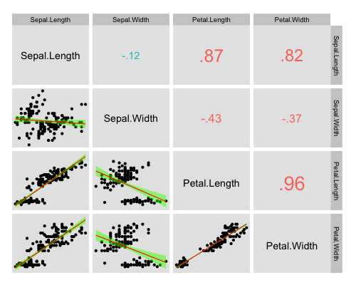
ggcorplot(
  data = iris[1:4],
  var_text_size = 5,
  cor_text_limits = c(5,10))
panel.cor <- function(x, y, digits=2, prefix="", cex.cor)
{
    usr <- par("usr"); on.exit(par(usr))
    par(usr = c(0, 1, 0, 1))
    r <- abs(cor(x, y))
    txt <- format(c(r, 0.123456789), digits=digits)[1]
    txt <- paste(prefix, txt, sep="")
    if(missing(cex.cor)) cex <- 0.8/strwidth(txt)

    test <- cor.test(x,y)
    # borrowed from printCoefmat
    Signif <- symnum(test$p.value, corr = FALSE, na = FALSE,
                  cutpoints = c(0, 0.001, 0.01, 0.05, 0.1, 1),
                  symbols = c("***", "**", "*", ".", " "))

    text(0.5, 0.5, txt, cex = cex * r)
    text(.8, .8, Signif, cex=cex, col=2)
}

pairs(iris[1:4], lower.panel=panel.smooth, upper.panel=panel.cor)

> system.time(pairs(iris[1:4]))
   user  system elapsed
  0.138   0.008   0.156
> system.time(splom(~iris[1:4]))
   user  system elapsed
  0.003   0.000   0.003
> system.time(plotmatrix(iris[1:4]))
   user  system elapsed
  0.052   0.000   0.052
> system.time(ggcorplot(
+ data = iris[1:4],
  var_text_size = 5,
  cor_text_limits = c(5,10)))

   user  system elapsed
  0.130   0.001   0.131
> system.time(pairs(iris[1:4], lower.panel=panel.smooth, upper.panel=panel.cor))
   user  system elapsed
  0.170   0.011   0.200
To leave a comment for the author, please follow the link and comment on their blog: Recology.
R-bloggers.com offers daily e-mail updates about R news and tutorials about learning R and many other topics. Click here if you're looking to post or find an R/data-science job.
Want to share your content on R-bloggers? click here if you have a blog, or here if you don't.