Last year, I spent a morning trying to return to first principles when modeling loss reserves. (Brief aside to non-actuaries: a loss reserve is the financial provision set aside to pay for claims which have either not yet settled, or have not yet been reported. If that doesn’t sound fascinating, this will likely be a fairly dull post.) I start by structuring the data in non-triangular format; that is the development lag is a columnar variable, rather than listing lags by column. This also allows me to store more than one observation for each combination of accident and development year, effectively storing multiple “triangles” in a single dataframe. That’s hardly novel; the ChainLadder package for R has functions to support switching the data from one to the other.

I pick incremental paid losses as the response variable and model it against prior cumulative losses. As a first cut, I just observe the scatter plot and see what it suggests. Below is that plot for Allstate’s workers comp portfolio of liabilities. The data is taken from the fantastic set compiled by Glenn Meyers and Peng Shi found here. I alter the column names and compute incremental and prior cumulative values.

GetTriangleData = function (dataSetName = "ppauto_pos.csv")
{
  URL.stem = "http://www.casact.org/research/reserve_data/"
  URL = paste(URL.stem, dataSetName, sep="")
  
  df = read.csv(URL)
  colnames(df) = c("GroupCode"
                   , "GroupName"
                   , "AccidentYear"
                   , "DevelopmentYear"
                   , "DevelopmentLag"
                   , "CumulativeIncurred"
                   , "CumulativePaid"
                   , "IBNR"
                   , "DirectEP"
                   , "CededEP"
                   , "NetEP"
                   , "Single"
                   , "Reserve1997")
  
  df = CalculateIncrementals(df, df$GroupName, df$AccidentYear, df$DevelopmentLag)
  return(df)
}

CalculateIncrementals = function(df, ...)
{
  df = df[order(...),]
  
  rownames(df) = NULL
  
  df$IncrementalPaid = df$CumulativePaid
  df$IncrementalIncurred = df$CumulativeIncurred
  df$PriorCumulativePaid = df$CumulativePaid
  df$PriorCumulativeIncurred = df$PriorCumulativeIncurred
  
  nrows = length(df$CumulativePaid)
  
  df$PriorCumulativePaid[2:nrows] = df$CumulativePaid[1:nrows-1]
  df$PriorCumulativeIncurred[2:nrows] = df$CumulativeIncurred[1:nrows-1]
  df$IncrementalPaid[2:nrows] = df$CumulativePaid[2:nrows] - df$CumulativePaid[1:nrows-1]
  df$IncrementalIncurred[2:nrows] = df$CumulativeIncurred[2:nrows] - df$CumulativeIncurred[1:nrows-1]
  
  firstLag = which(df$DevelopmentLag == 1)
  df$IncrementalPaid[firstLag] = df$CumulativePaid[firstLag]
  df$IncrementalIncurred[firstLag] = df$CumulativeIncurred[firstLag]
  df$PriorCumulativePaid[firstLag] = 0
  df$PriorCumulativeIncurred[firstLag] = 0
  
  return(df)
}

df = GetTriangleData("wkcomp_pos.csv")
bigCompany = as.character(df[which(df$CumulativePaid == max(df$CumulativePaid)),"GroupName"])
print(bigCompany)

df.sub = subset(df, GroupName == bigCompany)

df.sub = subset(df.sub, DevelopmentYear <=1997)

df.CL = subset(df.sub, DevelopmentLag != 1)
plt = ggplot(df.CL, aes(x = PriorCumulativePaid, y = IncrementalPaid, size=5)) + geom_point(show_guide=F)
print(plt)

LagFactor = as.factor(df.CL$DevelopmentLag)
plt = ggplot(df.CL, aes(x = PriorCumulativePaid, y = IncrementalPaid, legend.position="none", group = LagFactor, size=5, colour = LagFactor, fill = LagFactor)) + geom_point(show_guide=F)
print(plt)

plt = ggplot(df.CL, aes(x = PriorCumulativePaid, y = CumulativePaid, group = LagFactor, size=5, colour = LagFactor, fill = LagFactor)) + geom_point(show_guide=F)
print(plt)

Here’s what the Allstate data looks like:

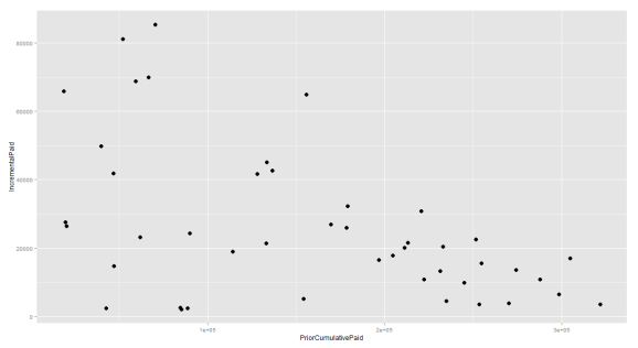
Notice that it appears as though any linear trend will be negative. Although this is somewhat intuitive (the more losses you pay, the less you’ll have to pay in the future), it doesn’t smell right. Mind, it doesn’t smell right because actuaries have had it beat into their heads that age-to-age development factors describe a line which runs through the origin. To restore our faith in what we’ve been taught, here’s what happens when we group that data based on development lag. The groupings are reflected by color:

If we fit a line to every set of points grouped by development lag, we now presume a positive slope, but one which decreases as lag increases.

What we have here is a multivariate regression, wherein the predictors are selected based on development lag. There are two papers that have been instrumental in getting me to grasp that in practical terms. The first is “Chain-Ladder Bias: Its Reason and Meaning” by Leigh Halliwell. It’s absolutely indispendable. The second was “Bootstrap Modeling: Beyond the Basics” by Shapland and Leong. Because I’m a very simple guy, it takes hours and hours of reading and deep thought to get to something very simple. That simple thing was the construction of a design matrix to represent the loss reserving model. Once you’ve got that, fitting a model becomes incredibly easy.

CreateDesignMatrixByCategory = function(Predictor, Category, MinFrequency)
{
    z = as.data.frame(table(factor(Category)))
    nCols = length(which(z$Freq >= MinFrequency)) + 1
    nRows = length(Predictor)
    DesignMatrix <- as.data.frame(matrix(0, nRows, nCols))
    for (i in 1:(nCols-1))
    {
        idx = array(FALSE, nRows)
        idx[which(Category==z[i,1])] = TRUE
        DesignMatrix[idx, i] = Predictor[idx]
    }
    
    idx = array(FALSE,nRows)
    tail = z[which(z$Freq < MinFrequency), 1]
    idx[which(Category %in% tail)] = TRUE
    DesignMatrix[idx, nCols] = Predictor[idx]
    
    dmNames = as.character(z[which(z$Freq >= MinFrequency), 1])
    dmNames = c(dmNames, "tail")
    colnames(DesignMatrix) = dmNames
    DesignMatrix = as.matrix(DesignMatrix)
    return (DesignMatrix)
}

So, it’s a bit ugly and I’m sure that it could be made to look a bit cleaner. Basically, all that we’re doing is the following: count the number of categories and produce an empty matrix with that many columns. You’ll provide one row for each observation. For a 10×10 loss triangle, that’s 55 rows. Fill the matrix with the predictor variable each time you match on the category.

For a traditional reserving model, the category will be development lags. Note that this means a very sparse design matrix. For a 10×10 triangle, the design matrix will have 550 elements, but only 55 of them will be filled. If you’re doing multiplicative chain ladder, it’s even fewer as the ten observations for lag 1 can’t be predicted.

I have a parameter to ensure that I get a minimum number of observations. I do this to smooth estimation for the tail factor, though it could have other applications. This means that if I have one observation for a particular lag in the tail, I can pool it with others.

I also create a set of weights for the regression. This allows me to switch between simple average development factors, weighted average or “pure” linear model factors. Daniel Murphy could explain this to you in his sleep. His 1994 paper is absolutely required reading and can do more justice to the subject than I can. Read this link.

CreateRegressionWeights = function(DesignMatrix, delta)
{
    RegressionWeights = rowSums(DesignMatrix)
    RegressionWeights = pmax(RegressionWeights,1)

    RegressionWeights=1/(RegressionWeights^delta)
    return (RegressionWeights)
}

I play fast and loose with the delta parameter and I’m never sure if I’m consistent with the literature. So, delta=0 -> pure linear, delta=1 -> weighted average and delta=2 -> simple average.

Once the design matrix and weights are in place, how do we calculate the link ratios? So damn easy.

dm <- CreateDesignMatrixByCategory(df.CL$PriorCumulativePaid, df.CL$DevelopmentLag, 2)
RegressionWeights <- CreateRegressionWeights(dm, 0)
Fit = lm(df.CL$IncrementalPaid ~ dm + 0, weights=RegressionWeights)
summary(Fit)

And that’s it. The fit object holds loads of diagnostic information to help you evaluate whether or not the model you’ve assumed is appropriate. In this instance, we find that the first three model factors are quite significant, after which parameter error begins to assert itself. R-squared looks fairly good, though there are a number of caveats about that metric. At some point in the near future, I’ll be ranting about heteroskedasticity.