Time-Series Policy Evaluation in R
Want to share your content on R-bloggers? click here if you have a blog, or here if you don't.
Quantifying the success of government policies is clearly important. Randomized control trials, like those conducted by drug companies, are often described as the ‘gold-standard’ for policy evaluation. Under these, a policy is implemented in/to one area/group (treatment), but not in/to another (control). The difference in outcomes between the two areas or groups represents the effectiveness of the policy.
Unfortunately, there many circumstances in which governments introduce policies and are not able to measure how are well, if at all, they work. A good example of this is childhood vaccinations against disease, since it is unethical to deny some children a potentially life-saving treatment. This makes evaluating these policies difficult, because there is no counterfactual event, i.e. everyone gets the treatment (in this case vaccination).
However, it is possible to evaluate the effectiveness of certain policies with time-series econometrics. For this example, I am going to use a series of monthly road death statistics in Ireland over the period 2003 to present. In November 2011, a new drink driving law was introduced which lowered the blood-alcohol limits. How has the introduction of this law changed road fatalities?
To evaluate this policy, I estimated a simple state space model using the R package sspir. The code I used for this example is almost exactly like the van drivers example in this paper. The following generalized linear model is assumed: Po(y_{t}) = a_{t} + b(LAW) + S_{t}, where the number of deaths, y_{t}, is a Poisson process that depends on a random walk, a_{t}, time-varying seasonal patterns, S_{t}, and the introduction of the law. The b parameter is the measure of the policy’s effect.
The usefulness of this model for policy evaluation, compared to an OLS linear regression for example, stems from the time-varying intercept a_{t}. In effect, this parameter substitutes the counterfactual or control group that we would need in a randomized control trial because it takes into account the underlying trend in the time-series before the policy change. The law dummy variable adds a shift to the underlying trend, acting as the relevant treatment effect.
A full overview of the state space system, and estimation using the Kalman filter is beyond the scope of this blog post. Interested readers should consult this paper and the references therein. The code to generate these results is below.
> head(road)
  deaths drinkdrive ind
1     20          0   1
2     21          0   2
3     33          0   3
4     23          0   4
5     28          0   5
6     37          0   6

mle <- function(psi) {
  m1 <- ssm(deaths ~ tvar(1) + drinkdrive + tvar(sumseason(time,12)),
            family=poisson(link="log"), data=road,
            phi=c(1,exp(psi)),C0=diag(13)*1000)
  m1fit <- getFit(m1)
  return(extended(m1fit)$likelihood)
}

res1 <- optim(par=c(0,0),fn=mle,method=c("L-BFGS-B"),
              control=list(fnscale=-1),hessian=FALSE)
The first part of the code sets up the state space system inside a function. The reason for this is to calculate the signal-to-noise ratio, which I call psi, using maximum likelihood. The signal-to-noise ratio dictates the ‘wiggliness’ of the random walk a_{t}. Too much signal will result in a_{t} matching the series exactly. Too little, and the random walk will collapse to a constant term, as in OLS. A similar argument can be made for the time-varying seasonal patterns.
After calculating the signal-to-noise ratio, I estimated the model with the maximum likelihood parameters. The function ssm automatically runs the iterated Kalman smoother, which provides the relevant information.
# estimate with mle pars
m2 <- ssm(deaths ~ tvar(1) + drinkdrive + tvar(sumseason(time,12)),
          family=poisson(link="log"), data=road,
          phi=c(1,exp(res1$par)),C0=diag(13)*1000)
m2fit <- getFit(m2)

100 * (exp(m2fit$m[1,2])-1) # effect of drink driving law

# calculate sd
m2sd <- NULL
for (i in 1:length(road$deaths)) {
  thisone <- m2fit$C[[i]][1:2,1:2]
  if (road$drinkdrive[i]==0) {
    m2sd <- c(m2sd,sqrt(thisone[1,1]))
  }
  else
    m2sd <- c(m2sd,sqrt(sum(thisone)))
}

# plot
road$ind <- 1:112
plot(road$ind,road$deaths,ylim=c(0,50),col="red",type="l",axes=F,
     xlab="Year",ylab="Death Count",main="Monthly Road Deaths, Ireland")
lines(exp(road$drinkdrive*m2fit$m[,2] + m2fit$m[,1]),col="blue")
lines(exp(road$drinkdrive*m2fit$m[,2] + m2fit$m[,1]+2*m2sd),lty=2,col="blue")
lines(exp(road$drinkdrive*m2fit$m[,2] + m2fit$m[,1]-2*m2sd),lty=2,col="blue")
abline(v=107)
axis(1, at=c(1,25,49,73,97), lab=c("2003","2005","2007","2009","2011"))
axis(2)
box()
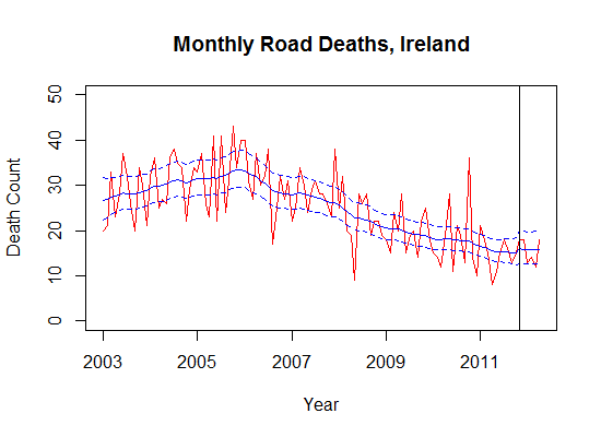
The following is a plot showing the underlying series (red), the policy relevant effect (shift in the blue line, black vertical line represents the policy change), and uncertainty (blue dotted lines). Perhaps it is too early to suggest this policy was ineffective. However, as is evident in the graph, this policy change did not result in less road deaths. In fact, this policy actually led to a 5.6% increase in road deaths, although a large amount of uncertainty surrounds these estimates, as shown by the 95% confidence intervals.
While I use this as an example, I should be clear that I do not condone driving under the influence of alcohol, nor do I think this was a bad policy. These data may not be a perfect measure of the policy’s effectiveness. Perhaps there are other time-series, like head-on collisions, for which the policy did make a discernable difference. Additionally, there may be previous policy changes in the series which I am unaware of.
R-bloggers.com offers daily e-mail updates about R news and tutorials about learning R and many other topics. Click here if you're looking to post or find an R/data-science job.
Want to share your content on R-bloggers? click here if you have a blog, or here if you don't.

