
Temperature reconstruction with useless proxies
Want to share your content on R-bloggers? click here if you have a blog, or here if you don't.
In a number of previous posts I considered the temperature proxies that have been used to reconstruct global mean temperatures during the past millenium. In this post I want to show how such a temperature reconstruction would look like if the proxies had no relation at all to the actual temperatures.
The motivation is the observation that the proxies are only weakly correlated with the temperatures during the observation period 1850-2000. Furthermore, standard Lasso regression which has been used in the past for temperature reconstruction is sensitive to spurious correlations due to autocorrelated inputs. And some of the over 1200 proxies are autocorrelated. Thus, in case the relation between proxies and temperatures is indeed nonexistent, that is if proxies had no predictive power about past temperatures, the lasso would still find “relevant” predictors and will happily fit a model to the observations. In this short post, I want to check how such a “reconstruction” based on useless proxies would typically look like.
I use the actually observed annual Northern hemisphere average temperatures (check this post to see where to get them):
    load("data_instrument.Rdata")
    t.nh <- instrument$CRU_NH_reform
I further assume that each of the K=1200 proxies is actually a realization of an AR(1) process of length N=1000 with uniformly distributed positive AR parameter and no causal relation to the observed temperatures:
    proxies <- lapply(seq(K),function(z) {
         arima.sim(model=list(order=c(1,0,0),ar=runif(1)),n=N) })
    proxies <- apply(as.matrix(proxies),1,unlist)
I fit a cross-validated Lasso model to the temperature observations, using the above pseudoproxies as inputs:
    library(glmnet)
    i.tr <- seq( N-length(t.nh)+1, N )
    lasso.model <- cv.glmnet(x=proxies[i.tr,],y=as.matrix(t.nh))
    coefz <- as.matrix(coef(lasso.model,s=lasso.model$lambda.min))
    recon <- cbind(rep(1,N),proxies) %*% coefz
For the plot below, the experiment was repeated 100 times with different AR(1) realizations. The temperature observations of the past 150 years are shown in red.
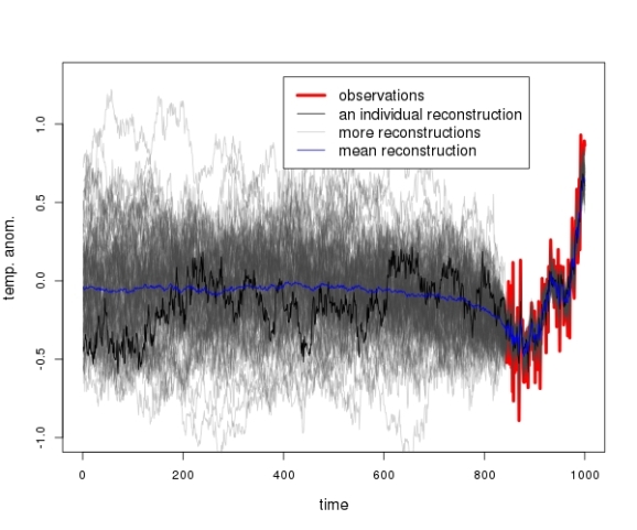
Even though the proxies are completely unrelated to the observations, the Lasso picks out a couple of them and reconstructs the observed temperatures almost perfectly. Every time!
In a lot of cases the reconstruction provides the impression as if there had been a “little ice age”, that is a period of anomalously low temperatures, before the start of the observation period in the mid-19th century.
In about 95 percent of the cases, the temperatures observed during the past 10 years or so would be deemed the highest during the past millenium. The hockeystick shape is the typical shape if proxies have no predictive power.
Conclusions
I do not doubt that global mean temperatures have gone up during the past decade. The data speaks for itself. Neither do I want to ridicule the climate scientist’s honest attempts at learning about past climate.
But I consider the predictive power of the proxies (tree rings, ice cores, beetle skeletons in sediments) to be limited at best. The above experiment shows that the conclusions in the heavily-cited climate change literature would be similar if all the proxies were in fact useless.
The usual conclusion that temperatures have never been as high as they are today might as well be based on spurious statistical effects. I hope for the field of climate science that this is not the case.
Complete R code:
library(glmnet)

#read data
load("data_instrument.Rdata")
t.nh <- instrument$CRU_NH_reform

#produce matrix of 1200 ar1 pseudo proxies
#and use them to reconstruct past temperatures
#repeat experiment 100 times
i.tr <- seq( N-length(t.nh)+1, N )
N <- 1000
K <- 1200
r <- matrix(nrow=0,ncol=N)
for (i in seq(100)) {
    proxies <- lapply(seq(K),function(z) {
	arima.sim(model=list(order=c(1,0,0),ar=runif(1)),n=N) })
    proxies <- apply(as.matrix(proxies),1,unlist)
    lasso.model <- cv.glmnet(x=proxies[i.tr,],y=as.matrix(t.nh))
    coefz <- as.matrix(coef(lasso.model,s=lasso.model$lambda.min))
    recon <- cbind(rep(1,N),proxies) %*% coefz
    r <- rbind(r,t(as.matrix(recon)))
}

#plot
par(cex.lab=1.2)
plot(i.tr,t.nh,xlim=c(0,N),ylim=c(-1,1.3),type="l",lwd=4,col="red", xlab="time",ylab="temp. anom.")
lapply( seq(100), function(z) {
    lines(seq(N),r[z,],col="#44444444") })
lines(seq(N),r[1,])
lines(colMeans(r),col="blue")
legend(x=400,y=1.3,c("observations","an individual reconstruction", "more reconstructions","mean reconstruction"),col=c("red","black","#44444444","blue"),lty=rep(1,4),lwd=c(4,1,1,1),cex=1.2)
R-bloggers.com offers daily e-mail updates about R news and tutorials about learning R and many other topics. Click here if you're looking to post or find an R/data-science job.
Want to share your content on R-bloggers? click here if you have a blog, or here if you don't.