
Rapidminer + R Example for Trading
[This article was first published on a Physicist in Wall Street, and kindly contributed to R-bloggers]. (You can report issue about the content on this page here)
Want to share your content on R-bloggers? click here if you have a blog, or here if you don't.
RapidMiner + R is an advanced tool that can be used to analyze trading strategies, In order to check its power I made a simple example using an algorithm based on a support vector machine for predicting the next day’s price and based on it I generated buying and selling signals. I have integrated quant indicators, SVM, and inally the strategy is evaluated. Want to share your content on R-bloggers? click here if you have a blog, or here if you don't.
The requirements needed to build the model are, of course, RapidMiner, Weka extension, time series extension and the R extension. This requires installing R with quantmod, TTR and PerformanceAnalytics packages. There is a thread to solve any problem here
To be able to reproduce my results I will detail each of the modules of the following figure:

1. R Process.
The objective is to process data from Yahoo finance and build the most common indicators to add to the series, these indicators have been taken considering the following article.To this end, here is a new paper written by an engineering student at UC Berkeley which uses “support vector machine” together with 10 simple technical indicators to predict the SPX index, purportedly with 60% accuracy
The content of the process is detailled here:
***********************************************
library(quantmod)
library(TTR)
library(PerformanceAnalytics)
# pull IBM data from Yahoo Finance
getSymbols(“IBM”,from=”2003-01-01″)
# Introduce RSI Indicator
IBM$RSI2 = RSI(Cl(IBM), 2)
#Introduce Eponential Moving Average indicator
IBM$EMA7=EMA(Cl(IBM), n=7, wilder=FALSE, ratio=NULL)
IBM$EMA50=EMA(Cl(IBM), n=50, wilder=FALSE, ratio=NULL)
IBM$EMA200=EMA(Cl(IBM), n=200, wilder=FALSE, ratio=NULL)
#Introduce MACD indicator
IBM$MACD26=MACD(Cl(IBM), nFast=12, nSlow=26, nSig=9)
#Introduce ADX indicator
IBM$ADX14=ADX(IBM, n=14)
#results <-transform(IBM,RSI.IBM=RSI(Cl(IBM), 2),RETURN=ret ,TIME=as.character(index(IBM)))
# remove 2003,2004,2005 in order to avoid NaN from EMA indicators
# To maintain time it is necessary to conver in texts
results <-transform(IBM["2006-01-01::2009-01-01"],TIME=as.character(index(IBM["2006-01-01::2009-01-01"])))
***********************************************
The output of the system is:

2. String to Time (Nominal to Date)
We convert date string to Date.

3. Close adjuste to Label
We put label the IBM adjusted close value in order to predict one day in advance..

4. set Time to ID (Set Role)
We use the TIME as ID for time serie data.
5. Widowing
We move one day in the future the variable to predict and add 2 new columns with lagged values in a time window of 2 days.

6. % sliding Window Validation

Time series validation

We use the Support Vector Machine Weka implementation

You can improve the accuracy of the prediction algorithm using any parameter optimizer or attribute selection.
Now Validation process
7.. Obtain Technical Test data
This module is similar to the first one except we use evaluation data from the last year
***********************************************
library(quantmod)
library(TTR)
library(PerformanceAnalytics)
# pull IBM data from Yahoo Finance
getSymbols(“IBM”,from=”2009-01-01″)
# Introduce RSI Indicator
IBM$RSI2 = RSI(Cl(IBM), 2)
#Introduce Eponential Moving Average indicator
IBM$EMA7=EMA(Cl(IBM), n=7, wilder=FALSE, ratio=NULL)
IBM$EMA50=EMA(Cl(IBM), n=50, wilder=FALSE, ratio=NULL)
IBM$EMA200=EMA(Cl(IBM), n=200, wilder=FALSE, ratio=NULL)
#Introduce MACD indicator
IBM$MACD26=MACD(Cl(IBM), nFast=12, nSlow=26, nSig=9)
#Introduce ADX indicator
IBM$ADX14=ADX(IBM, n=14)
#results <-transform(IBM,RSI.IBM=RSI(Cl(IBM), 2),RETURN=ret ,TIME=as.character(index(IBM)))
# remove 2009 in order to avoid NaN from EMA indicators 2010 evaluation
# To maintain time it is necessary to conver in texts
results <-transform(IBM["2010-01-01::"],TIME=as.character(index(IBM["2010-01-01::"])))
.
***********************************************
We use a similar pre-process Flow..

11. Apply Model
We will apply the model obtained before
And finally we analyze the trading strategy results
12. Prediction Lable as Regular (Set Role)
It is modified the predicted label to use inside R process.
13. Date to Nominal
It is modified the date to nominal to use it in R process.
14. Set TIME as Regular (Set Role)
It is modified the TIME attributte as a regular to use it in R process..
15. Set TIME as Regular (Set Role)
This script is inspired in FOSS trading code.
***********************************************
library(quantmod)
library(TTR)
library(PerformanceAnalytics)
# 31 prediction close_ROCel
# 33 close_ROCel
close_ROC <- ROC(data[33])
dates = as.Date(data$TIME)
prediction_ROC <-ROC(data[31])
close_ROC[1] <- 0
prediction_ROC[1] <- 0
#generate signals from prediction values
sigup <- ifelse(prediction_ROC > 0, 1, 0)
sigdn <- ifelse(prediction_ROC < 0, -1, 0)
# Replace missing signals with no position
# (generally just at beginning of series)
sigup[is.na(sigup)] <- 0
sigdn[is.na(sigdn)] <- 0
sig <- sigup + sigdn
# Calculate equity curves
eq_up <- cumprod(1+close_ROC*sigup)
eq_dn <- cumprod(1+close_ROC*sigdn)
eq_all <- cumprod(1+close_ROC*sig)
# obtain result
result <-transform(data,sig=sig ,ret=close_ROC, eq_up=eq_up, eq_dn=eq_dn, eq_all=eq_all)
# This function gives us some standard summary
# statistics for our trades.
tradeStats <- function(signals, returns) {
# Inputs:
# signals : trading signals
# returns : returns corresponding to signals
# Combine data and convert to data.frame
sysRet <- signals * returns * 100
posRet <- sysRet > 0 # Positive rule returns
negRet <- sysRet < 0 # Negative rule returns
dat <- cbind(signals,posRet*100,sysRet[posRet],sysRet[negRet],1)
dat <- as.data.frame(dat)
# Aggreate data for summary statistics
means <- aggregate(dat[,2:4], by=list(dat[,1]), mean, na.rm=TRUE)
medians <- aggregate(dat[,3:4], by=list(dat[,1]), median, na.rm=TRUE)
sums <- aggregate(dat[,5], by=list(dat[,1]), sum)
colnames(means) <- c("Signal","% Win","Mean Win","Mean Loss")
colnames(medians) <- c("Signal","Median Win","Median Loss")
colnames(sums) <- c("Signal","# Trades")
all <- merge(sums,means)
all <- merge(all,medians)
wl <- cbind( abs(all[,"Mean Win"]/all[,"Mean Loss"]),
abs(all[,”Median Win”]/all[,”Median Loss”]) )
colnames(wl) <- c("Mean W/L","Median W/L")
all <- cbind(all,wl)
return(all)
}
# trade stats
stats<- as.data.frame(tradeStats(sig,close_ROC))
ret_all<-close_ROC
xts.ts <- xts(ret_all,dates)
drawdownrport = table.Drawdowns(xts.ts)
***********************************************
In the following graph you can see the not well ROC of this strategy
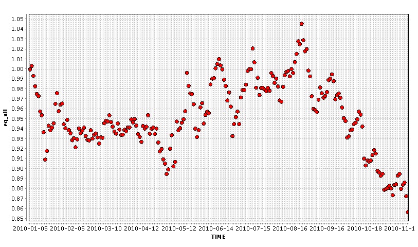
Return obtained during buy and shell signals

This strategy is a simplification, and that should be understand as a proof of concept.
All information is in this tutorial, however if you want to
To leave a comment for the author, please follow the link and comment on their blog: a Physicist in Wall Street.
R-bloggers.com offers daily e-mail updates about R news and tutorials about learning R and many other topics. Click here if you're looking to post or find an R/data-science job.
Want to share your content on R-bloggers? click here if you have a blog, or here if you don't.