Picturing Trees
Want to share your content on R-bloggers? click here if you have a blog, or here if you don't.
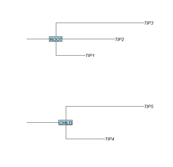
In this post I like to illustrate the R package “ape” for phylogenetic trees for the purpose of assembling trees. The function read.tree creates a tree from a text description. For example the following code creates and displays two elementary trees:
require(ape)
tree.top <- (read.tree(text = "(TIP1:1,TIP2:2,TIP3:3):1;"))
tree.top$node.label <- "ROOT"
par(mfrow=c(2,1))
plot(tree.top,cex=1,srt=0,direction="r",root.edge=TRUE)
nodelabels(tree.top$node.label,frame="r",cex=1)

tree.child <- (read.tree(text = "(TIP4:1,TIP5:2):1;"))
tree.child$node.label <- "CHILD"
plot(tree.child,cex=1,srt=0,direction="r",root.edge=TRUE)
nodelabels(tree.child$node.label,frame="r",cex=1)
The required syntax for the read.tree text input is ( TIP_NAME : TIP_BRANCH_LENGTH , … ) : ROOT_BRANCH_LENGTH;
Note that for better illustration in the example above the length are chosen differently for the branches that lead to each leaf or tip.
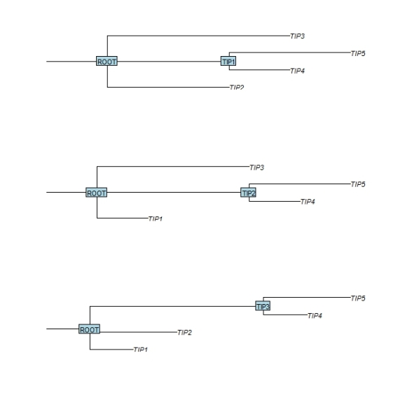
Next the function bind.tree is used to attach the child tree to the root tree. The argument where determines the position within the parent root tree where the child branch should be attached. In the first example below the child branch is attached to the branch of the ‘TIP1″ leaf. In this process the receiving leaf label is replaced by the new branch. In order to retain the receiving leaf label, I set the node.label attribute of the incoming child tree to its name.
par(mfrow=c(3,1))

tree.child$node.label <- "TIP1"
tree.combined <- bind.tree(tree.top, tree.child, where=which(tree.top$tip.label == tree.child$node.label ), position=0)
plot(tree.combined,cex=1,srt=0,direction="r",root.edge=TRUE)
nodelabels(tree.combined$node.label,frame="r",cex=1)

tree.child$node.label <- "TIP2"
tree.combined <- bind.tree(tree.top, tree.child, where=which(tree.top$tip.label == tree.child$node.label ), position=0)
plot(tree.combined,cex=1,srt=0,direction="r",root.edge=TRUE)
nodelabels(tree.combined$node.label,frame="r",cex=1)

tree.child$node.label <- "TIP3"
tree.combined <- bind.tree(tree.top, tree.child, where=which(tree.top$tip.label == tree.child$node.label ),position=0)
plot(tree.combined,cex=1,srt=0,direction="r",root.edge=TRUE)
nodelabels(tree.combined$node.label,frame="r",cex=1)
This procedure of adding branches to leafs can be repeated to build more and more complex trees. Happy gardening !
R-bloggers.com offers daily e-mail updates about R news and tutorials about learning R and many other topics. Click here if you're looking to post or find an R/data-science job.
Want to share your content on R-bloggers? click here if you have a blog, or here if you don't.


